Leaflet, GeoTIFF, and Colormaps

Using {leaflet} with a GeoTIFF background layer and resolving difficulties with RGB colormaps
R
Data visualization
Published

February 21, 2025

Documenting how to generate a colormap for a geo-encoded TIFF layer into a leaflet map.

TL;DR

colorvec <- terra::coltab(terra::rast(geotiff_file))[[1]] |> 
  mutate(rgb = rgb(red, green, blue, alpha, maxColorValue = 255)) |> 
  pull(rgb)

# And within the `leafem::addGeotiff()` function, add the argument:
leafem::addGeotiff(
  colorOptions = colorOptions(
    palette = colorvec,
    domain = c(0, 255)
  )

Background

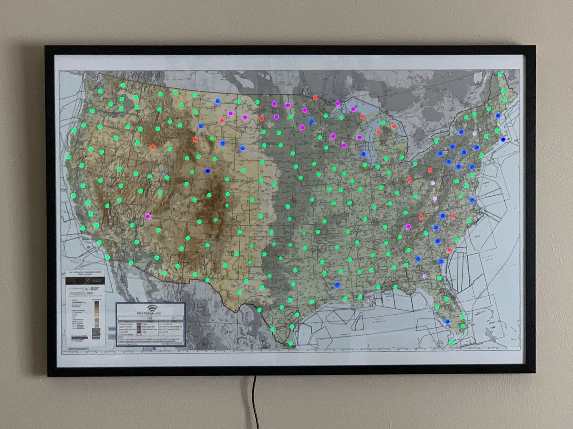
I’ve seen some advertisements for nice framed or shadowboxed aviation VFR sectional charts with RGB LED’s set in them to display flight categories (VFR / MVFR / IFR / LIFR), including this one on Etsy (a bargain at $500, compared to another one at $2,050).

For a little while, I thought I’d make one myself, probably driven by a Raspberry Pi or Arduino, but… code is faster and more flexible.

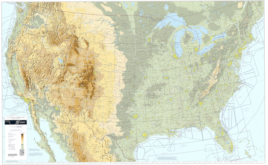
VFR sectional map in geoTIFF format source

The FAA provides VFR raster charts that are in geo-encoded TIFF format. The one for the entire conterminous United States is under the Planning tab as the U.S. VFR Wall Planning Geo-Tiff (Zip). It’s rather large at~60 MB.

It comes with a metadata file with a lot of data source information but is sparse on the TIFF encoding details:

The file is 300 dots per inch and 8-bit color. The data is provided as a GeoTIFF.

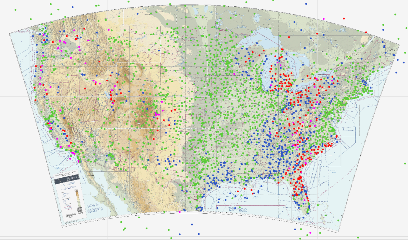
It does also give the latitude / longitude bounds, which I use to filter the METAR data in the next step.

METAR weather data source

The federal Aviation Weather Center offers all current METAR observations in updated every minute in one compressed CSV file.

# df_raw <- read_csv("https://aviationweather.gov/data/cache/metars.cache.csv.gz", skip = 5)
load("df_raw.rda")

df <- df_raw |>
  mutate(
    flight_category = factor(flight_category, levels = c("LIFR", "IFR", "MVFR", "VFR"), order = TRUE)
  ) |> 
  filter(
    !is.na(flight_category),
    !is.na(latitude),
    !is.na(longitude),
    # from chart metadata HTML
    between(latitude, 21.550541, 51.747171),
    between(longitude, -129.917883, -64.138074)
  ) |> 
  transmute(
    station_id, flight_category, latitude, longitude, raw_text
  )

df |> head(n = 5)
# A tibble: 5 × 5
  station_id flight_category latitude longitude raw_text                        
  <chr>      <ord>              <dbl>     <dbl> <chr>                           
1 MMIO       LIFR                25.5    -101.  MMIO 201310Z RTD 00000KT 1/2SM …
2 KXER       VFR                 27.9     -91.0 KXER 201310Z AUTO 35010G20KT 31…
3 CYMO       MVFR                51.3     -80.6 CYMO 201309Z AUTO 28005KT 5SM -…
4 CYNM       LIFR                49.8     -77.8 CYNM 201308Z AUTO 34008KT 3/4SM…
5 CYMT       IFR                 49.8     -74.5 CYMT 201308Z AUTO 33008KT 290V3…

Plotting in leaflet

Everything’s going smoothly! Let’s put it together in a leaflet plot.

# Flight category color palette
pal <- colorFactor(
  palette = c("#FF00FF", "#FF0A0A", "#2D55C8", "#59CC38"),
  domain = c("LIFR", "IFR", "MVFR", "VFR"),
  ordered = TRUE)

hover_labels <- as.list(paste(df$flight_category, " - ", df$raw_text))
geotiff_file <- "us_vfr.tif"

df |> 
  leaflet() |>
  leafem::addGeotiff(
    file = geotiff_file,
    resolution = 300,
    opacity = 0.7,
    rgb = TRUE,
  ) |>
  addCircleMarkers(
    ~longitude, ~latitude,
    radius = 5,
    stroke = FALSE,
    color = ~pal(flight_category),
    fillOpacity = 1,
    label = hover_labels
  ) |> 
  addLegend(
    position = "bottomright",
    pal = pal,
    values = ~flight_category,
    title = "Flight Category"
  )

Hmmm, what happened to the map colors?

TIFF color maps

After much Google searching and fighting with ChatGPT, I learned a few things.

RGB files usually have 3 bands, one each for Red, Green, and Blue. When I checked using a function from the terra package:

terra::rast("us_vfr.tif")
#> class       : SpatRaster 
#> dimensions  : 11441, 18509, 1  (nrow, ncol, nlyr)
#> resolution  : 262.4775, 262.4655  (x, y)
#> extent      : -2189361, 2668836, -1471398, 1531470  (xmin, xmax, ymin, ymax)
#> coord. ref. : Wall_Planning_Chart 
#> source      : us_vfr.tif 
#> color table : 1 
#> name        : us_vfr

…I found that the TIFF file had only 1 band (nlyr = 1).

In retrospect, it makes sense. The TIFF metadata said it was only 8-bit (256 distinct colors). If you look closely, you’ll see the color table : 1 – that’s another hint that instead of encoding a full (R, G, B) (and maybe even alpha), there’s a color lookup table someplace.

After more Google-fu:

colormap <- terra::coltab(terra::rast(geotiff_file))[[1]]

head(colormap, n = 10)
#>    value red green blue alpha
#> 1      0 255   255  255   255
#> 2      1 255   255    0   255
#> 3      2 255     0  255   255
#> 4      3 255     0    0   255
#> 5      4   0   255  255   255
#> 6      5   0   255    0   255
#> 7      6   0     0  255   255
#> 8      7   0     0    0   255
#> 9      8 255   255    1   255
#> 10     9 252   252  254   255

Looks a lot like a dataframe for a color lookup table

  • value ranges from 0 to 255
  • three more columns of red, green, and blue, all with values from 0 to 255
  • alpha is always 255 (makes sense for normal RGB files)

So somehow, the leafem::addGeotiff() function will need to get this color lookup incorporated.

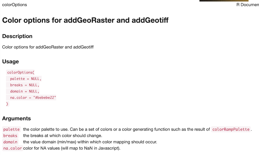
Looks like there’s an argument called colorOptions, which sounds promising, but all it says is list defining the palette, breaks and na.color to be used. Not very helpful documentation.

More Google-fu, showed that there’s also a function called colorOptions. Let’s get help on that function.

So…

  • everything defaults to NULL
  • the palette argument is the palette
  • the breaks argument is the breaks
  • the domain is the domain (min/max)

That’s… not at all helpful.

I don’t even remember what bizarre guesswork and trial-and-error eventually led me to the solution.

I figured out that palette had to encode a function that would convert the index of the lookup table into some sort of color representation, which I guessed might be a hex code color representation.

The “function” ended up working fine as simply a vector of color values, since indexing into that vector looks like passing an argument into a function which yields the color value output. I worried that R uses 1-based indexing but the values in the lookup table started at 0, but it ended up being fine, presumably because of the domain argument of min/max.

So here’s the code that fixed the color mapping:

colormap <- coltab(rast(geotiff_file))[[1]]

colorvec <- colormap |> 
  mutate(rgb = rgb(red, green, blue, alpha, maxColorValue = 255)) |> 
  pull(rgb)
  
head(colorvec, n = 10)
#>  [1] "#FFFFFFFF" "#FFFF00FF" "#FF00FFFF" "#FF0000FF" "#00FFFFFF" "#00FF00FF"
#>  [7] "#0000FFFF" "#000000FF" "#FFFF01FF" "#FCFCFEFF"

df |> 
  leaflet() |>
  leafem::addGeotiff(
    file = geotiff_file,
    resolution = 300,
    opacity = 0.7,
    colorOptions = colorOptions(
      palette = colorvec,  # Custom color function
      domain = c(0, 255)
    ),
    rgb = TRUE,
  )

Success…

It really didn’t take much code to get it to work, but for someone with zero background in colorspaces and how they’re described, it wasn’t really easy finding explanations what to do. Worked out in the end though!