METAR analysis, part 2 – Incidental Findings

TL;DR

Newly deployed shinylive app that runs in the client browser to allow interactive review and analysis of METAR data at a number of different airports. Access the app at https://jhchou.github.io/metar_analysis/. Comment here if you’d like any other airports added.

This won’t be an explanatory post so much as a quick list of technical improvements to the previously described analysis, of 20+ years of hourly METAR (Meteorological Aerodrome Report) weather data.

(someplace over Walpole, MA back in September 2024)

Previous workflow:

Airport metadata from AirNav.com
- airport name, runway headings, and time zones
- time zones ended up non-ideal; changed when accessed during daylight savings time
Weather data from Iowa Environmental Mesonet
- data was accessed for each airport by manual web page form request
- 20 years of hourly data in CSV ASCII text typically around 70 MB of data
Analysis within a Quarto dashboard
- generated manually, one HTML dashboard per airport
- did not use R Shiny because of lack of access to a Shiny server

New approach

R riem package
- for programmatic access to Iowa Environmental Mesonet (IEM)
- source of additional airport metadata (GPS location, stable timezone)
- dev build allows access of just the fields needed
- saving more limited data as serialized R instead of CSV text decreased size of 20 years of hourlyt data from 70 MB to ~3.5 MB per airport
R shinylive is amazing
- Shiny allows interactive analysis, so can allow modification of personal weather minimums with immediate analysis feedback
- allows serving a Shiny app as a static web page
- R/Shiny all compiled under WebAssembly to run in the client – no server needed
R leaflet
- airport location metadata easily obtained from IEM metadata
- shinylive allows interactivity
- use leaflet and shiny in conjunction for a nice way to select airports with available data
Deployed to GitHub pages as a static web page
- shinylive runs client-side
- smaller airport data files are reasonable to keep on GitHub
- programmatic access makes it trivial to add airports

Bottom line – really nice improvement

from manual analysis of one airport at a time generating single airport HTML dashbaords
to an easily deployed Shiny app with multiple airports available and real-time analysis

Airport selection screen

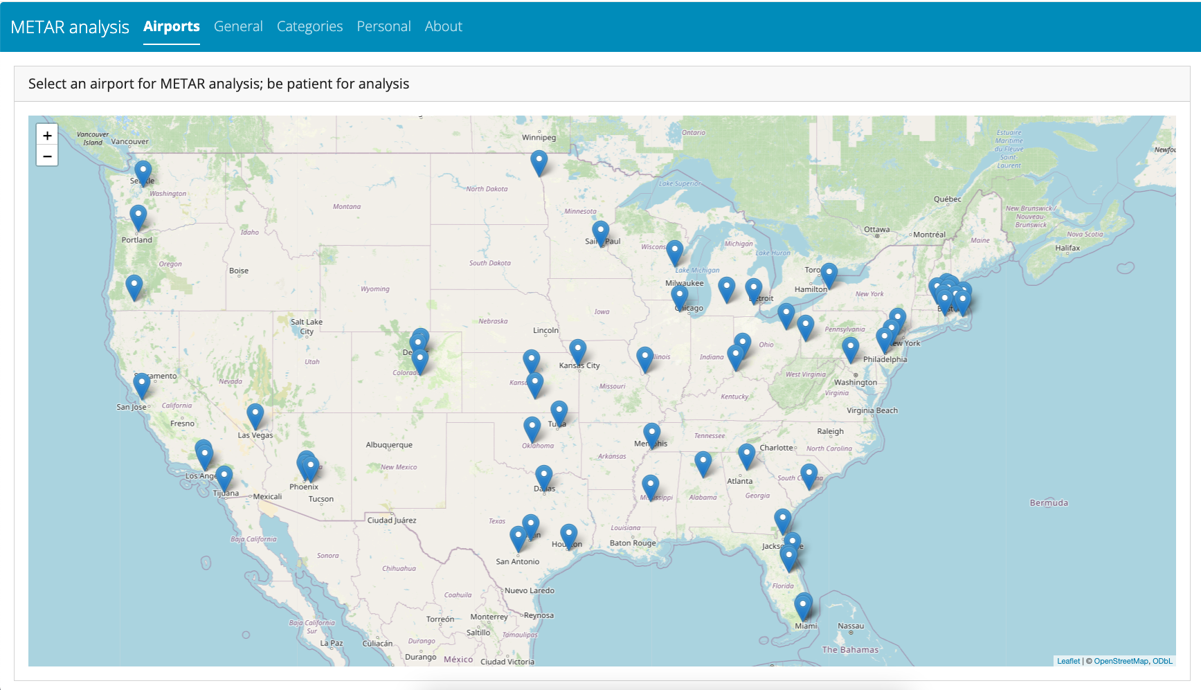
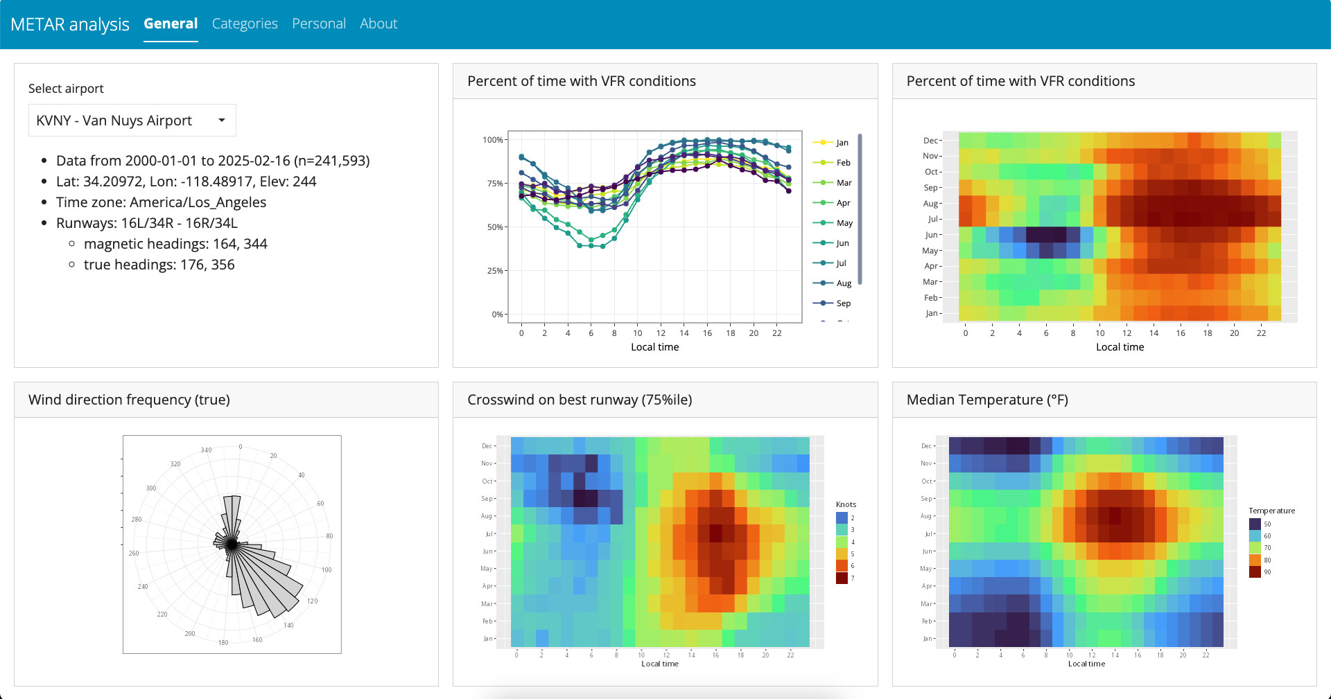
First of 3 tabs presenting results

`riem` package

A few details on using riem an R package to access data from the Iowa Environmental Mesonet.

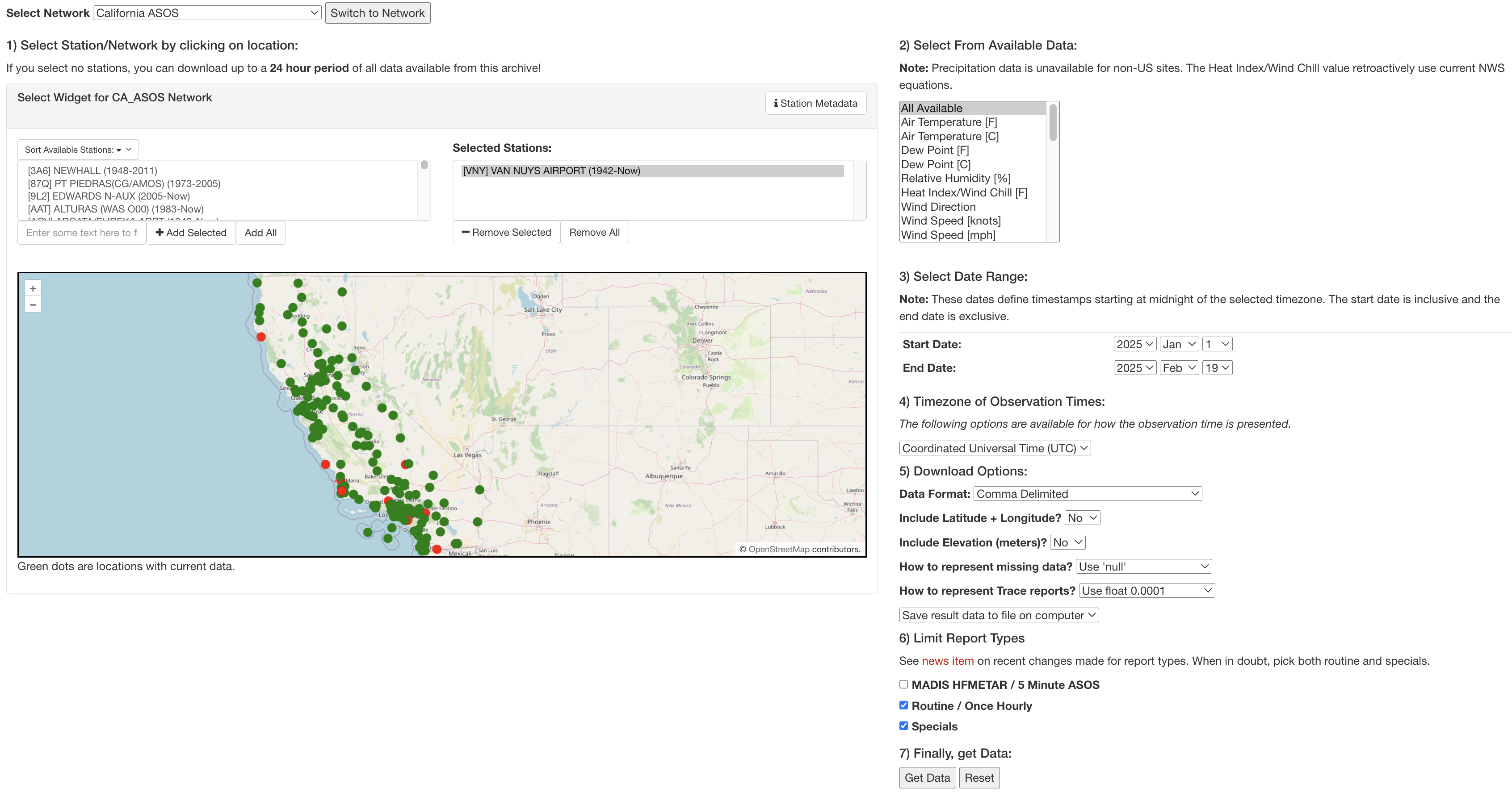
My first iteration of the tool required manual selection of form inputs to select the proper ASOS network, the specific airport, and details of download options. This was already pretty tedious, so I also selected “All Available” (even though I didn’t use all the data).

When downloaded as a text CSV file, 20 years of data was ~70 MB per airport, and the manual steps were a hindrance to adding additional airports to analyze.

When I came across riem, much better programmatic solutions became possible. For a given airport, you need to know which “ASOS network” (typically a state) had the data you wanted.

The riem::riem_networks() function gives the codes for all 264 of the networks.

# Identify IA Mesonet networks
networks <- riem_networks() # 264 networks
networks |> head(n=10) |> knitr::kable()

code	name
AE__ASOS	United Arab Emirates ASOS
AF__ASOS	Afghanistan ASOS
AG__ASOS	Antigua and Barbuda ASOS
AI__ASOS	Anguilla ASOS
AK_ASOS	Alaska ASOS
AL__ASOS	Albania ASOS
AL_ASOS	Alabama ASOS
AM__ASOS	Armenia ASOS
AN__ASOS	Netherlands Antilles ASOS
AO__ASOS	Angola ASOS

Likewise, the riem::riem_stations() function gives all the ASOS reporting stations available within that network.

# Identify reporting stations wihin a network
stations <- riem_stations("MA_ASOS")
names(stations)
#>  [1] "index"         "id"            "synop"         "name"         
#>  [5] "state"         "country"       "elevation"     "network"      
#>  [9] "online"        "county"        "climate_site"  "wfo"          
#> [13] "modified"      "spri"          "tzname"        "iemid"        
#> [17] "archive_begin" "metasite"      "ugc_county"    "ugc_zone"     
#> [21] "ncdc81"        "ncei91"        "longitude"     "latitude"     
#> [25] "wigos"         "archive_end"   "plot_name"     "lon"          
#> [29] "lat"

I don’t generally like to blindly scrape websites, but it was helpful to get a list of all airports within each network. I wrote a bit of code that looped over the 264 networks and archived all the station metadata into a dataframe for future use.

To fetch the actual data, you use the riem::riem_measures() function. I initially used dev version via because the CRAN version wasn’t initially able to limit the data fields returned, but it looks like a version was released 2025-01-31 that supports it now.

The valid time for each row of weather data is reported in UTC time, but the timezone name is available in the previously obtained metadata as tzname, so it’s easy to convert to local times (needed for the use I wanted).

Simple function to fetch a from a given network’s station ID, just the fields I wanted, from a given start date, making some fields more compact by factorizing, and returning it as an R dataframe. The resulting data size when saved as a serialized R object (via saveRDS and readRDS) was much smaller, down from ~70 MB to ~3.5 MB.

get_mesonet <- function(network, id, tzname, start_date) {
  riem::riem_measures(
    # skyc4 and skyl4 seem to be unpopulated, but keep just in case some stations have
    station = id, # station is case-sensitive, OWD worked; owd and kowd did not
    date_start = start_date, # date_end not required
    data = c("tmpf", "drct", "sknt", "vsby", "gust",
      "skyc1", "skyc2", "skyc3", "skyc4", "skyl1", "skyl2", "skyl3", "skyl4"),
    elev   = FALSE, # have from metadata
    latlon = FALSE, # have from metadata
    report_type = c("routine", "specials")
  ) |> 
    mutate(
      local = with_tz(valid, tzone = tzname), # tzname from metadata
      across(c(skyc1:skyc4), as.factor)
    )
}

Fetching new data from an airport has become trivial thanks to riem!

For fun

Let’s plot all available stations from the archived metadata within a box enclosing the conterminous United States.

library(tidyverse)
library(leaflet)

load("airports_mesonet.rda") # airports_mesonet

df <- airports_mesonet |>
  filter(
    online, # currently active?
    between(latitude, 24.5, 49.4), # Conterminous US
    between(longitude, -125, -67)  # Conterminous US
  ) |> 
  select(id, name, network, latitude, longitude)

hover_labels = as.list(paste(df$id, " - ", str_to_title(df$name), " - ", df$network))

df |> 
  leaflet() |>
  addTiles() |>
  addCircleMarkers(
    ~longitude, ~latitude,
    radius = 1,
    fillOpacity = 1,
    label = hover_labels
  )