I was notified recently about the availability of “expanded” tables of parameters for the WHO Growth Standards that are much more fine-grained than the ones that I’ve used in the past. The resolution is at the daily rather than monthly level.
The primary purpose of the expanded tables seems to be less for clinical use and more for generating very high resolution growth chart plots for “national health cards”.
Countries that need to incorporate the WHO charts into existing national health cards have to locally reproduce the charts to fit the format of the health cards. These expanded tables are required to reproduce growth charts with adequate precision. They provide: a) the centiles with 3 decimal precision; b) age in days for age-based indicators; c) additional centiles.
Although I thought it unlikely to be of significance for clinical (or even research) use, once I know there’s a dataset out there, it’s really hard not to play with it.
However, there were a total of 18 additional charts and copying and pasting the chart parameters out of that many source documents sounded really tedious. So, what could have been maybe an hour of copy-pasting became several hours of coding. Such is the life of a coder.
This post describes the partial automation of data-scraping of the expanded WHO Growth Standard parameters.

Source Files
The WHO makes available the parameter tables in Excel format, at the bottom of each growth standard’s web page, as “Expanded tables for constructing national health cards.” I manually downloaded each of the 18 files and put them in a single standards directory.
filenames <- list.files("standards")
filenames
[1] "acfa-boys-zscore-expanded-tables.xlsx"
[2] "acfa-girls-zscore-expanded-tables.xlsx"
[3] "bfa-boys-zscore-expanded-tables.xlsx"
[4] "bfa-girls-zscore-expanded-tables.xlsx"
[5] "hcfa-boys-zscore-expanded-tables.xlsx"
[6] "hcfa-girls-zscore-expanded-tables.xlsx"
[7] "lhfa-boys-zscore-expanded-tables.xlsx"
[8] "lhfa-girls-zscore-expanded-tables.xlsx"
[9] "ssfa-boys-zscore-expanded-table.xlsx"
[10] "ssfa-girls-zscore-expanded-table.xlsx"
[11] "tsfa-boys-zscore-expanded-tables.xlsx"
[12] "tsfa-girls-zscore-expanded-tables.xlsx"
[13] "wfa-boys-zscore-expanded-tables.xlsx"
[14] "wfa-girls-zscore-expanded-tables.xlsx"
[15] "wfh-boys-zscore-expanded-tables.xlsx"
[16] "wfh-girls-zscore-expanded-tables.xlsx"
[17] "wfl-boys-zscore-expanded-table.xlsx"
[18] "wfl-girls-zscore-expanded-table.xlsx" What’s pretty cool is that there is pretty clear naming convention and each Excel file has the same overall structure. In each file:
- first column represents the continuous variable on the X-axis (age in days, except for the Weight for Length/Height charts, which are in cm)
- second through fourth columns are the L, M, and S parameters, to allow calculation of Z-scores via the Cole LMS method
- (the other columns are redundant – measurement values for a few specified Z-scores or percentiles, all of which can be derived by the Cole method)
Converting tables to dataframes with some metadata
The filenames have a consistent structure as well, with the first two parts identifying the specific chart type (“wfa” is “weight for age”) and the second part identifies the sex.
We can split the filenames and use a simple dictionary convert the chart types into the same naming convention I already use in my R peditools package.
Next, iterate over each of the Excel files and convert them to R dataframes with columns compatible with pre-existing peditools columns.
lmsdata_list <- list() # list to store extracted LMS dataframes
for (i in 1:length(filenames)) {
  df <- read_excel(paste0("standards/", filenames[i])) %>% select(1:4) # age, L, M, S
  gender <- ifelse(parts[[i]][2] == "boys", "m", "f") # convert "boys" / "girls" to "m" / "f"
  chart_code <- parts[[i]][1] # e.g., acfa, bfa, hcfa, lhfa, ssfa, tsfa, wfa, wfh, wfl
  temp <- strsplit(parts[[i]][1], "f")
  measure <- measures[[temp[[1]][1]]] # before 'f' in chart_code
  age_type <- measures[[temp[[1]][2]]] # after 'f' in chart_code

  # Group charts together. Each group can have multiple measures
  # - HCFA, LHFA, WFA, (and BFA) all have age (x-axis) range from 0 to 1856 days
  # - ACFA, SFA, and TFA all have age (x-axis) range from 91 to 1856 days
  # - WFH (x-axis range 65-120 cm) and WFL (x-axis range 45-110 cm) are the ONLY non-age-based charts; will separate given different ranges
  chart = case_when( # group similar charts, which will have distinct "measures"
        chart_code %in% c("wfa", "hcfa", "lhfa", "bfa") ~ "who_expanded",
        chart_code %in% c("ssfa", "tsfa", "acfa") ~ "who_expanded_arm_skin",
        chart_code %in% c("wfl") ~ "who_wt_for_len",
        chart_code %in% c("wfh") ~ "who_wt_for_ht",
        .default = "ERROR"
  )

  age_units <- tolower(names(df)[1])
  age_units = case_when(
    age_units == "day" ~ "days",
    age_units %in% c("height", "length") ~ "cm"
  )
  names(df)[1] <- "age"
  measure_units = case_when(
        measure %in% c("arm_circ", "head_circ", "length_height") ~ "cm",
        measure %in% c("triceps", "subscapular") ~ "mm",
        measure == "bmi" ~ "kg/m2",
        measure == "weight" ~ "kg",
        .default = "ERROR"
  )

  df <- df %>%
    transmute(
      chart,
      age,
      age_units,
      gender,
      measure,
      measure_units,
      L, M, S
    )
  lmsdata_list[[i]] <- df
  print(paste0("Processed ", measure, " (", measure_units, ") for ", age_type, " (", age_units, ") - ", gender, " into ", chart))
}
[1] "Processed arm_circ (cm) for age (days) - m into who_expanded_arm_skin"
[1] "Processed arm_circ (cm) for age (days) - f into who_expanded_arm_skin"
[1] "Processed bmi (kg/m2) for age (days) - m into who_expanded"
[1] "Processed bmi (kg/m2) for age (days) - f into who_expanded"
[1] "Processed head_circ (cm) for age (days) - m into who_expanded"
[1] "Processed head_circ (cm) for age (days) - f into who_expanded"
[1] "Processed length_height (cm) for age (days) - m into who_expanded"
[1] "Processed length_height (cm) for age (days) - f into who_expanded"
[1] "Processed subscapular (mm) for age (days) - m into who_expanded_arm_skin"
[1] "Processed subscapular (mm) for age (days) - f into who_expanded_arm_skin"
[1] "Processed triceps (mm) for age (days) - m into who_expanded_arm_skin"
[1] "Processed triceps (mm) for age (days) - f into who_expanded_arm_skin"
[1] "Processed weight (kg) for age (days) - m into who_expanded"
[1] "Processed weight (kg) for age (days) - f into who_expanded"
[1] "Processed weight (kg) for height (cm) - m into who_wt_for_ht"
[1] "Processed weight (kg) for height (cm) - f into who_wt_for_ht"
[1] "Processed weight (kg) for length (cm) - m into who_wt_for_len"
[1] "Processed weight (kg) for length (cm) - f into who_wt_for_len"Checking the import
Finally, combine them all into a single dataframe and check it.
lmsdata_new <- bind_rows(lmsdata_list) # combine all into a single dataframe
lmsdata_new %>% count(chart, measure, measure_units, age_units) %>% knitr::kable()| chart | measure | measure_units | age_units | n |
|---|---|---|---|---|
| who_expanded | bmi | kg/m2 | days | 3714 |
| who_expanded | head_circ | cm | days | 3714 |
| who_expanded | length_height | cm | days | 3714 |
| who_expanded | weight | kg | days | 3714 |
| who_expanded_arm_skin | arm_circ | cm | days | 3532 |
| who_expanded_arm_skin | subscapular | mm | days | 3532 |
| who_expanded_arm_skin | triceps | mm | days | 3532 |
| who_wt_for_ht | weight | kg | cm | 1102 |
| who_wt_for_len | weight | kg | cm | 1302 |
Another quick sanity check is to plot all the charts out, one panel per chart group, one color per measure, plotting both genders. This figure is generated with plotly so it’s possible to interact with each panel.
library(plotly)

g <- lmsdata_new %>%
  arrange(age) %>%
  ggplot(aes(age, M, color = measure, group = gender)) +
  geom_line() +
  facet_wrap(~chart, scales = "free") +
  theme_bw()

ggplotly(g)
Comparison of monthly vs expanded daily parameterization
The expanded parameters really causes a huge increase in size of parameterization – these 18 charts have 27856 rows of data.
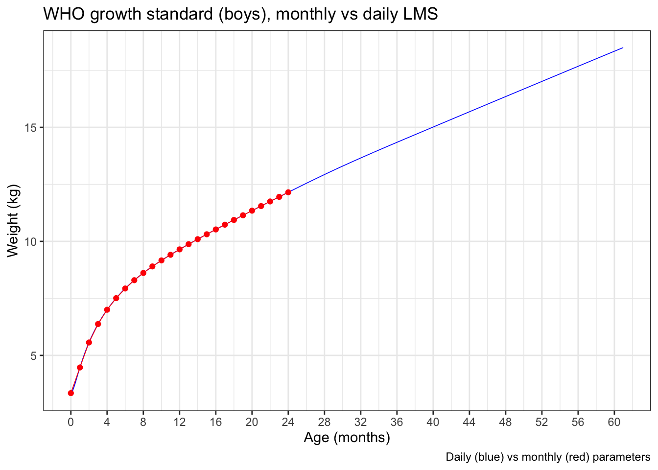
The expanded WHO weight-for-age growth standard for males includes 1857 rows of data for ages from 0 - 1856 days (0 - 61 months). In comparison, the 2006 WHO weight-for-age growth standard done monthly from 0 - 24 months has a total of only 25 rows.
Other than the expanded age range, is there much practical difference in the fine vs coarse parameterization?
Let’s compare the male weight-for-age charts. The red points are from the monthly parameterization, with linear interpolation between the 25 points. The blue line is from the daily parameters.
As expected, the differences at the macro level are negligible.
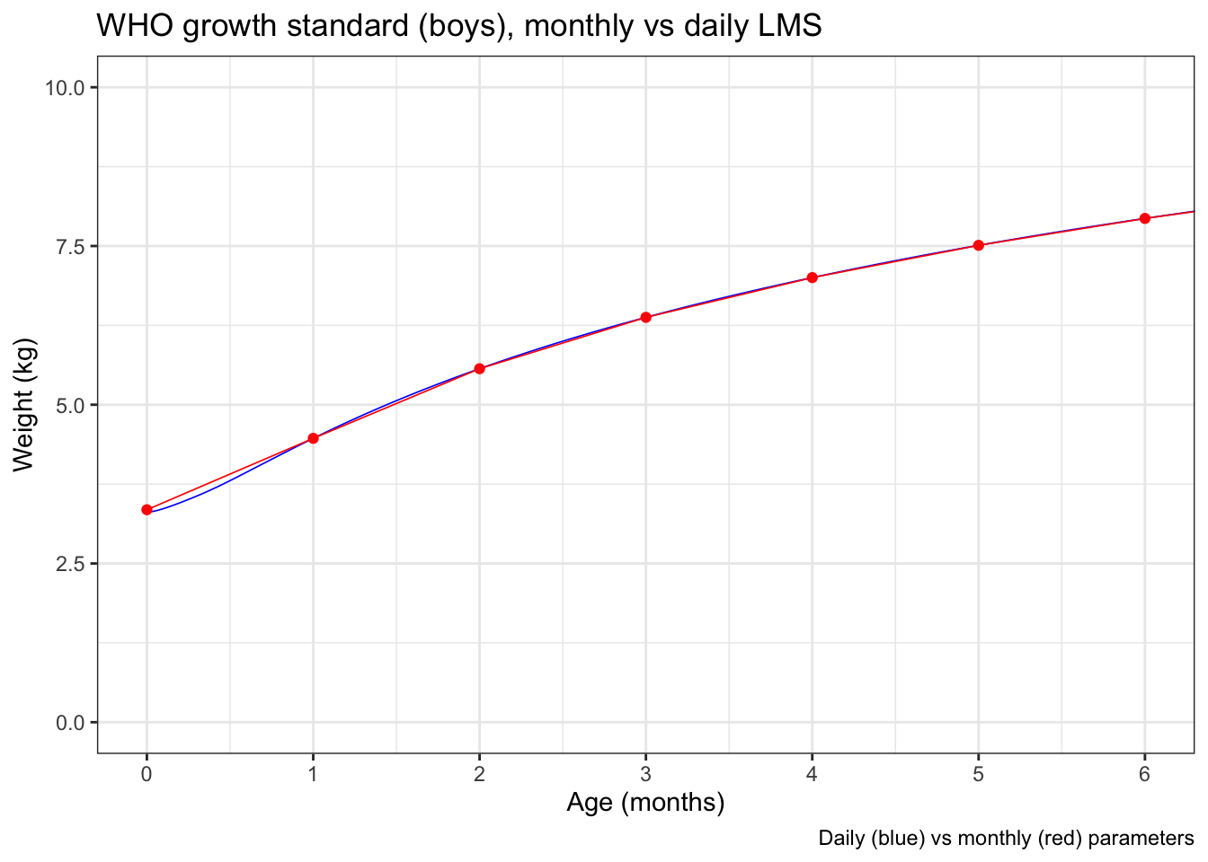
But zooming in to the first 6 months, where the curvature is greatest, you can detect a little bit of divergence between the daily (blue) and interpolated monthly (red) data.
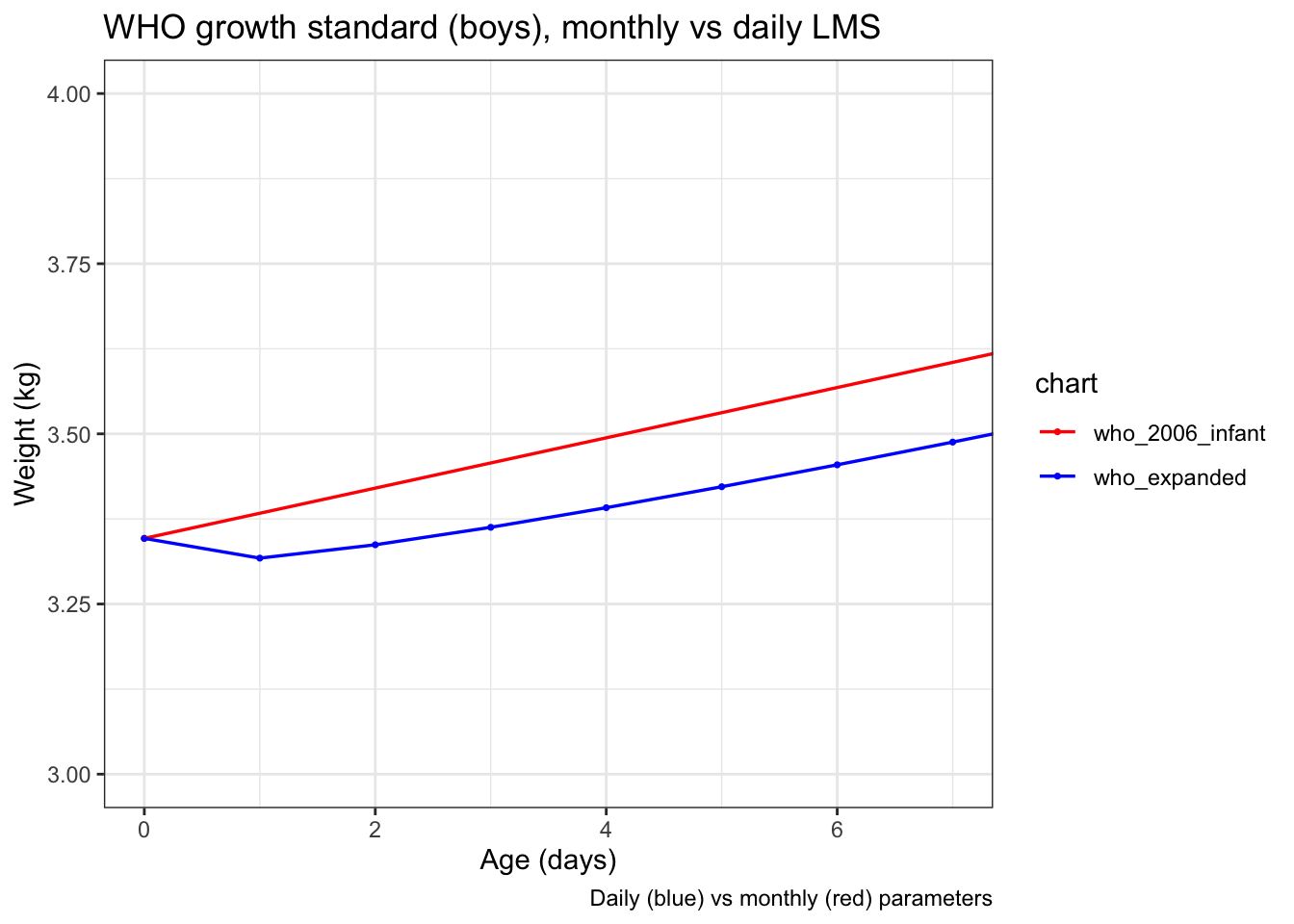
And if you zoom in REALLY far to just the first 7 days after birth, you can see that the WHO expanded weight-for-age actually has the median weight decrease of 29 grams from 3346.4* grams at birth to 3317.4 grams at age 1 day before starting to come up, reflecting the normal postnatal weight loss.
(*I include the full precision of the data in the expanded tables intentionally. While great for producing high quality graphics, this is an example of how silly it is to use high precision numbers in actual practice.)
Why you might NOT want to use the expanded tables
For background, first off, the WHO charts are meant for “term” babies. I’ve always found this problematic. If you define “term” as between 37 0/7 (beyond late preterm) and 41 6/7 weeks (before post-dates), there’s a pretty huge expected difference in size (and clinical risks).
Setting aside the problem of lumping all “term” babies together, some have suggested that the WHO charts can be used for former preterm babies by “correcting” to age relative to their due date.
But if you use the WHO expanded weight-for-age charts with age correction, these former preterm babies would be supposed to spontaneously have a median 29 gram weight loss the day after their due date, which is just silly.
Conclusion
The WHO Growth Standard expanded parameter tables are really nice to provide very smooth, high-resolution plots, but there isn’t really a strong indication to prefer them over the coarser parameterizations.
That being said, I’ve made calculations available via the WHO expanded parameters on my PediTools Universal: Bulk Calculator Shiny app, because… why not?