library(tidyverse)
library(corrplot)
library(randomForest)
library(knitr)
library(rgl) # for 3D scatterplot
knit_hooks$set(webgl = hook_webgl)
knitr::opts_chunk$set(cache=TRUE)
# setupKnitr()I share here the full code and output for an exploratory data visualization in R Markdown submitted for a contest in January 2017.
The code includes data exploration, feature generation / simplification, summary statistics, plotting distributions of predictors, assessment of correlations, and initial exploration of predictive modeling using random forests.
In January 2017, I had the pleasure of attending the 2017 ComputeFest, hosted by the Institute for Applied Computational Science at Harvard University. The skill-building workshops were excellent, including introductions to a number of topics, e.g.:
- Data Science in Python
- Introduction to MATLAB
- Data Science in Python
- Introduction to R, R Programming for Data Analysis
- Deep Learning for Image Segmentation with TensorFlow
There was also a contest in exploratory data visualization hosted by Prodigy Finance. From the contest instructions:
The idea here is to do exploratory visualization in preparation for data analysis. The dataset we will use is from the UCI machine learning repository: https://archive.ics.uci.edu/ml/datasets/Covertype. The dataset contains cartographic variables that might be useful in predicting the kind of tree cover. Your visualizations should be useful to an analyst in creating machine learning models to analyze this dataset: you are looking for correlations between the “features” and the kind of tree cover.
My wife and I decided to use this as an opportunity to practice our data exploration skills in R. It was quite a suprise when our submission was chosen as the winner – the prize was two Amazon Echos!
I share below our submission. Because it was produced using RMarkdown, it was a simple copy / paste to have it built with Quarto.
Edited to add in 2022-08: slight changes were made to the tidyverse code to remove deprecated functions like mutate_each and guide(<scale> = FALSE). Otherwise, the code is as submitted in 2017.
Without further ado:
Introduction
Exploratory visualization in preparation for data analysis, of the Covertype Data Set from the UCI machine learning repository with cartographic features for predicting the classes of tree cover.
Goals:
- look for correlations between the features and the kind of tree cover
- label axes clearly and caption and legend your images
- report which puts together these visualizations with some description in PDF or HTML format
As this is only for practice, a test set is not being set aside, as would be normal practice prior to exploratory data analysis in preparation for machine learning.
Dataset loading
The dataset consists of 581,012 rows with the target (forest cover type class) and 54 predictors consisting of 10 continuous variables and 44 factors. The 44 factors actually only represent one of four wilderness areas and one of forty soil types. The forty soil types, in-turn, specify a climatic zone and a geologic zone.
# d <- read.csv(file = 'covtype.data', header = FALSE)
# save(d, file = 'data.Rda')
load('data.Rda')

# Name                                     Data Type    Measurement                       Description
# Elevation                               quantitative    meters                       Elevation in meters
# Aspect                                  quantitative    azimuth                      Aspect in degrees azimuth
# Slope                                   quantitative    degrees                      Slope in degrees
# Horizontal_Distance_To_Hydrology        quantitative    meters                       Horz Dist to nearest surface water features
# Vertical_Distance_To_Hydrology          quantitative    meters                       Vert Dist to nearest surface water features
# Horizontal_Distance_To_Roadways         quantitative    meters                       Horz Dist to nearest roadway
# Hillshade_9am                           quantitative    0 to 255 index               Hillshade index at 9am, summer solstice
# Hillshade_Noon                          quantitative    0 to 255 index               Hillshade index at noon, summer soltice
# Hillshade_3pm                           quantitative    0 to 255 index               Hillshade index at 3pm, summer solstice
# Horizontal_Distance_To_Fire_Points      quantitative    meters                       Horz Dist to nearest wildfire ignition points
# Wilderness_Area (4 binary columns)      qualitative     0 (absence) or 1 (presence)  Wilderness area designation
# Soil_Type (40 binary columns)           qualitative     0 (absence) or 1 (presence)  Soil Type designation
# Cover_Type (7 types)                    integer         1 to 7                       Forest Cover Type designation

names(d) <- c(
    'elevation','aspect','slope','hydro_h','hydro_v','road_h','shade_09','shade_12','shade_15','fire_h',
    'wilderness_1','wilderness_2','wilderness_3','wilderness_4',
    paste0(c('soil_'), c(1:40)),
    'cover'
  )
Dataset pre-processing
The data preprocessing extracts the wilderness areas, soil types, climatic zones, and geologic zones, and replaces the category codes for with human-readable labels.
cover_types <- c('Spruce/Fir','Lodgepole Pine','Ponderosa Pine','Cottonwood/Willow','Aspen','Douglas-fir','Krummholz')
wilderness_areas <- c('Rawah', 'Neota', 'Comanche Peak', 'Cache la Poudre')

climate_zone <- c(2,2,2,2,2,2,3,3,4,4,4,4,4,5,5,6,6,6,7,7,7,7,7,7,7,7,7,7,7,7,7,7,7,7,8,8,8,8,8,8)
climatic_zones <- c('lower montane dry','lower montane','montane dry','montane','montane dry and montane','montane and subalpine','subalpine','alpine')
climate_zone <- climatic_zones[climate_zone]

geologic_zone <- c(7,7,7,7,7,7,5,5,2,7,7,7,7,1,1,1,1,7,1,1,1,2,2,7,7,7,7,7,7,7,7,7,7,7,7,7,7,7,7,7)
geologic_zones <- c('alluvium','glacial','shale','sandstone','mixed sedimentary','unspecified','igneous and metamorphic','volcanic')
geologic_zone <- geologic_zones[geologic_zone]

d <- d %>%
  mutate(
    id = row_number(),
    cover = cover_types[cover]
  )

d_soil <- d %>%
  select(id, starts_with('soil_')) %>%
  gather(key = 'soil_type', value = 'value', -id) %>%
  filter(value != 0) %>%
  select(-value) %>%
  mutate(
    soil_type = sub('soil_', '', soil_type) %>% as.numeric(),
    climate = climate_zone[soil_type],
    climate = factor(climate,
      levels = c('alpine','subalpine', 'montane and subalpine',
        'montane dry and montane', 'montane', 'montane dry', 'lower montane')),
    geologic = geologic_zone[soil_type]

  )

d_wilderness <- d %>%
  select(id, starts_with('wilderness_')) %>%
  gather(key = 'wilderness_type', value = 'value', -id) %>%
  filter(value != 0) %>%
  select(-value) %>%
  mutate(
    wilderness_type = sub('wilderness_', '', wilderness_type) %>% as.numeric(),
    wilderness_type = wilderness_areas[wilderness_type]
  )

d <- d[, c(1:10, 55, 56)] %>%
  inner_join(d_soil, by = 'id') %>%
  inner_join(d_wilderness, by = 'id') %>%
  mutate(across(11:16, factor)) %>%
  select(-id)
Initial univariate data exploration
Summary statistics
summary(d) elevation aspect slope hydro_h
Min. :1859 Min. : 0.0 Min. : 0.0 Min. : 0.0
1st Qu.:2809 1st Qu.: 58.0 1st Qu.: 9.0 1st Qu.: 108.0
Median :2996 Median :127.0 Median :13.0 Median : 218.0
Mean :2959 Mean :155.7 Mean :14.1 Mean : 269.4
3rd Qu.:3163 3rd Qu.:260.0 3rd Qu.:18.0 3rd Qu.: 384.0
Max. :3858 Max. :360.0 Max. :66.0 Max. :1397.0
hydro_v road_h shade_09 shade_12
Min. :-173.00 Min. : 0 Min. : 0.0 Min. : 0.0
1st Qu.: 7.00 1st Qu.:1106 1st Qu.:198.0 1st Qu.:213.0
Median : 30.00 Median :1997 Median :218.0 Median :226.0
Mean : 46.42 Mean :2350 Mean :212.1 Mean :223.3
3rd Qu.: 69.00 3rd Qu.:3328 3rd Qu.:231.0 3rd Qu.:237.0
Max. : 601.00 Max. :7117 Max. :254.0 Max. :254.0
shade_15 fire_h cover soil_type
Min. : 0.0 Min. : 0 Aspen : 9493 29 :115247
1st Qu.:119.0 1st Qu.:1024 Cottonwood/Willow: 2747 23 : 57752
Median :143.0 Median :1710 Douglas-fir : 17367 32 : 52519
Mean :142.5 Mean :1980 Krummholz : 20510 33 : 45154
3rd Qu.:168.0 3rd Qu.:2550 Lodgepole Pine :283301 22 : 33373
Max. :254.0 Max. :7173 Ponderosa Pine : 35754 10 : 32634
Spruce/Fir :211840 (Other):244333
climate geologic
alpine : 40437 alluvium : 20987
subalpine :401983 glacial : 92272
montane and subalpine : 8166 igneous and metamorphic:467469
montane dry and montane: 602 mixed sedimentary : 284
montane : 93593
montane dry : 284
lower montane : 35947
wilderness_type
Cache la Poudre: 36968
Comanche Peak :253364
Neota : 29884
Rawah :260796
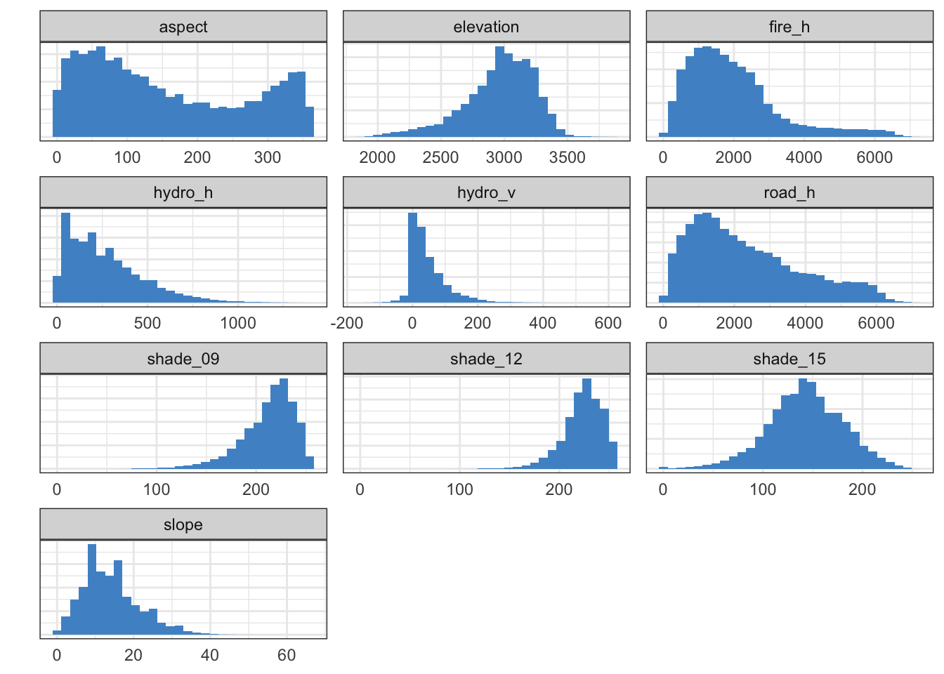
Distribution of the 10 continuous predictor variables
A plot of the distributions of all 10 continuous predictors (on different scales) confirms that each predictor has adequate variance.
d[, 1:10] %>%
  gather(key = measure, value = value) %>%
  ggplot(aes(value)) +
  geom_histogram(fill = 'steelblue3', bins = 30) +
  facet_wrap(~measure, scales = 'free', ncol = 3) +
  ylab('') +
  theme_bw() +
  theme(
    axis.text.y = element_blank(),
    axis.ticks = element_blank(),
    axis.title.x = element_blank()
  )
Marked class imbalance of prediction target
A histogram shows marked class imbalance of the seven forest cover categories. This is important to be aware of because of its potential to affect classifier training later on.
g <- d %>%
  ggplot(aes(cover, color = cover, fill = cover)) +
  geom_bar(alpha = 0.5) +
  labs(title = 'Frequency of Forest Cover Types in the Dataset', y = 'Frequency') +
  theme_bw() +
  guides(fill = "none", color = "none") +
  theme(
    axis.text.x = element_text(angle=45, hjust = 1),
    axis.title.x = element_blank()
  )
g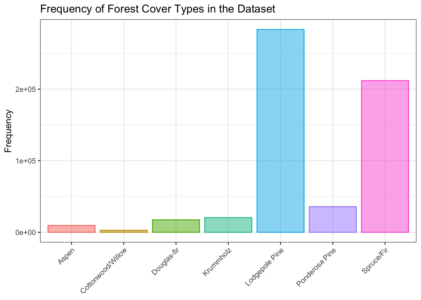
Multivariate data exploration
Assessment of correlation between numeric predictors
A correlation matrix of the 10 continuous predictor features shows some degree of correlation, both positive and negative, between some pairs of predictors, but overall there does not appear to be an excessive amount.
c <- cor(d[, 1:10])
corrplot(c, order = 'hclust', tl.cex = 0.75)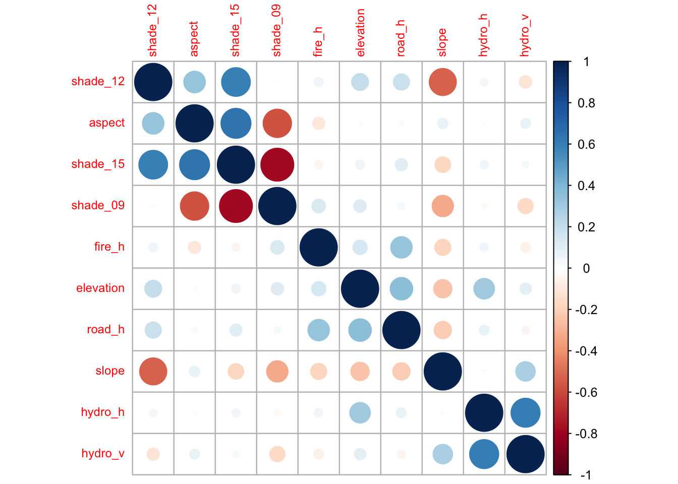
Pairwise analysis of continuous variables by balanced sampling
The following plot shows pairwise comparisons of each of the 10 continuous predictors with 30 randomly selected points from each of the 7 types of forest cover (color-coded). Selecting 30 at random from each of the forest covers counteracts the severe class imbalance, making it easier to see clusters of forest cover.
The plot works better on a large display, but is quite effective at demonstrating interesting associations between predictors as well as clustering of forest cover type as related to pairs of predictors.
Note the non-linear correlation between aspect or slope and the three shade-related features, which makes sense given the relationship between direction to sun + generation of shade by slope. Some of the U-shaped associations between the predictors are easily appreciated here, while not being apparent in the correlation matrix above.
# library(scales)
# show_col(hue_pal()(7)) # show the default ggplot2 color palette for 7 colors

d2 <- d[, c(1:11)] %>% group_by(cover) %>% sample_n(size = 30) # sample equal number from each class?a
d2[,c(1:10)] %>%
  pairs(
    main = 'Pairs plot of continuous predictors and forest cover type',
    pch = 21, cex = 0.55,
    bg = c('#F8766D','#C49A00','#53B400','#00C094','#00B6EB','#A58AFF','#FB61D7')[unclass(d2$cover)],
    col = alpha('#FFFFFF', 0.0), upper.panel = NULL)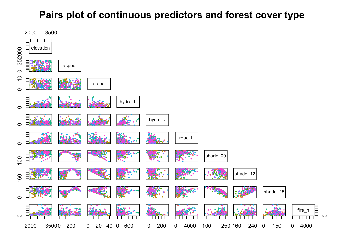
Correlations of target with predictors
Variation in distribution of forest cover by each predictor
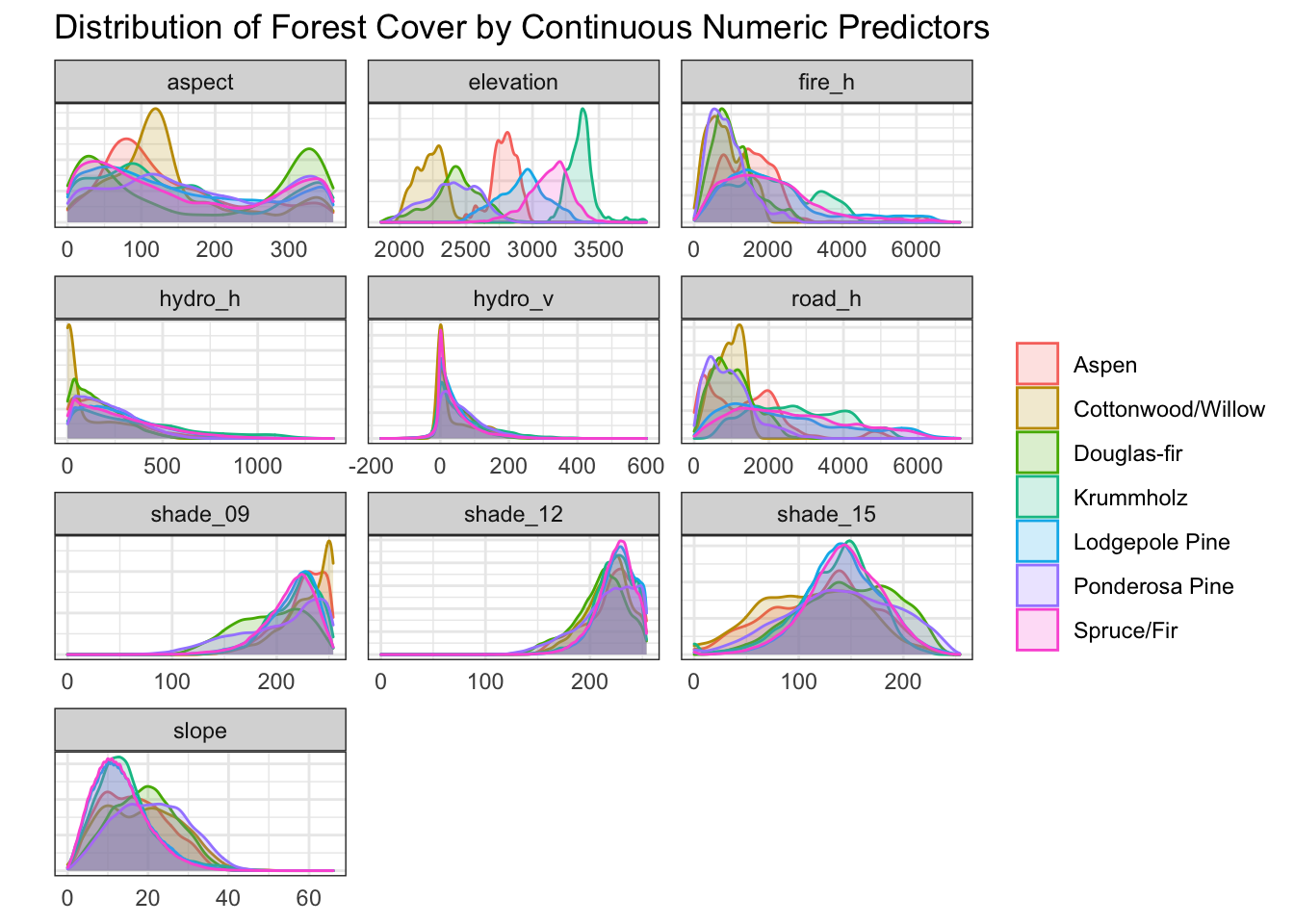
A density plot of each of the 7 classes of forest cover was examined for each of the 10 numeric predictors.
Some interesting features are immediately apparent; for example, in the panel for elevation, one can see that cottonwoods are predominantly found at lower elevations, aspens in the mid-range, and krummholz at higher elevations.
d[, c(1:11)] %>%
  gather(key = measure, value = value, -cover) %>%
  ggplot(aes(value, color = cover, fill = cover)) +
  geom_density(alpha = 0.2) + theme_bw() +
  facet_wrap(~measure, scales = 'free', ncol = 3) +
  labs(title = 'Distribution of Forest Cover by Continuous Numeric Predictors') +
  ylab('') +
  theme(
    axis.text.y = element_blank(),
    axis.ticks = element_blank(),
    axis.title.x = element_blank(),
    legend.title = element_blank()
    # legend.position = c(0.9, 0.1),  legend.justification = c("right", "bottom"),
    # legend.direction = "horizontal"
    )
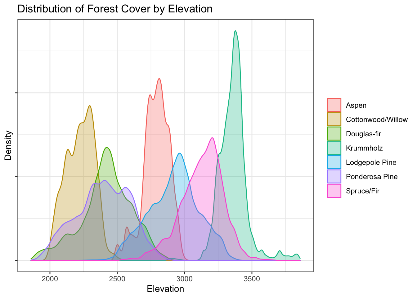
Elevation
d %>%
  ggplot(aes(elevation, fill = cover, color = cover)) +
  geom_density(alpha = 0.3) +
  labs(
    title = 'Distribution of Forest Cover by Elevation',
    x = 'Elevation', y = 'Density'
    ) +
  theme_bw() +
  theme(
    legend.title = element_blank(),
    axis.text.y = element_blank()
    )
Violin plot of distribution of cover types by numeric predictor
To reduce the effect of the overlapping density distributions, violin plots are another way to visualize the relationship between each type of forest cover and the continuous variables.
Elevation shows significantly more distinct profiles for the different forest cover types than any other single predictor.
d[, c(1:11)] %>%
  gather(key = measure, value = value, -cover) %>%
  ggplot(aes(cover, value, color = cover)) +
  geom_violin(aes(fill = cover), alpha = 0.5) +
#  geom_boxplot(width = 0.15) +
  facet_wrap(~measure, scales = 'free', ncol = 3) +
  labs(
    title = 'Distribution of forest cover by continuous numeric predictors',
    x = '', y = '') +
  theme_bw() +
  theme(
    axis.text.y = element_blank(), axis.text.x = element_blank(),
    axis.ticks = element_blank(), legend.title = element_blank())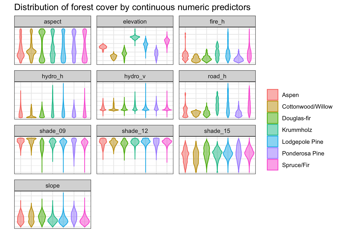
Density plot of cover by pairs of predictors
Visualizing forest cover types based on the density plot of two predictors shows better separation between forest cover types than with single predictors.
For the sake of space, only the density of forest cover with respect to elevation and fire point distance are shown, although other pairs of predictors were also assessed.
d %>% ggplot(aes(elevation, fire_h, color = cover)) +
  geom_density_2d() +
  facet_wrap(~cover) +
  labs(
    title = '2D-density of forest cover type by elevation and fire point distance',
    x = 'Elevation', y = 'Horizontal distance to fire points'
  ) +
  theme_bw() +
  guides(color = "none")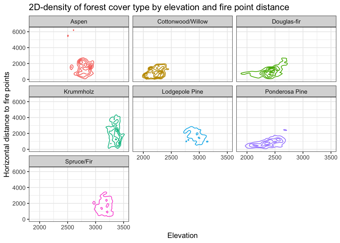
Interactive 3D scatter plot of forest cover by 3 predictors
Clustering of forest types can be appreciated upon rotation of the 3D scatterplot by 3 predictor features – elevation, aspect, and fire point distance. Again, to deal with the forest cover class imbalance, 60 of each forest class were randomly sampled from the dataset to ensure all classes are represented.
d2 <- d[, c(1:11)] %>% group_by(cover) %>% sample_n(size = 60)
with(d2,
plot3d(
elevation, aspect, fire_h,
type="s", size = 1.2,
col = c('#F8766D','#C49A00','#53B400','#00C094','#00B6EB','#A58AFF','#FB61D7')[unclass(cover)]
))
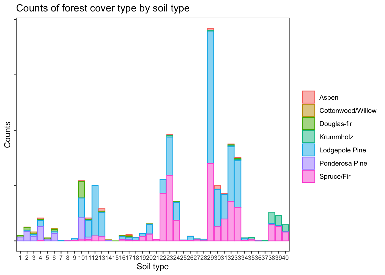
rglwidget()Absolute counts of forest cover types by soil type
The soil types representation is very unbalanced within the data set, as shown below. Because of this, the subsequent plots will show the proportions of each type of forest cover, within particular predictor classes.
d %>% ggplot(aes(soil_type, fill = cover, color = cover)) +
  geom_bar(alpha = 0.5) +
  theme_bw() +
  labs(
    title = 'Counts of forest cover type by soil type',
    x = 'Soil type', y = 'Counts'
    ) +
  theme(
    panel.grid = element_blank(),
    axis.text.x = element_text(size = 8),
    legend.title = element_blank(),
    axis.text.y = element_blank()
    )
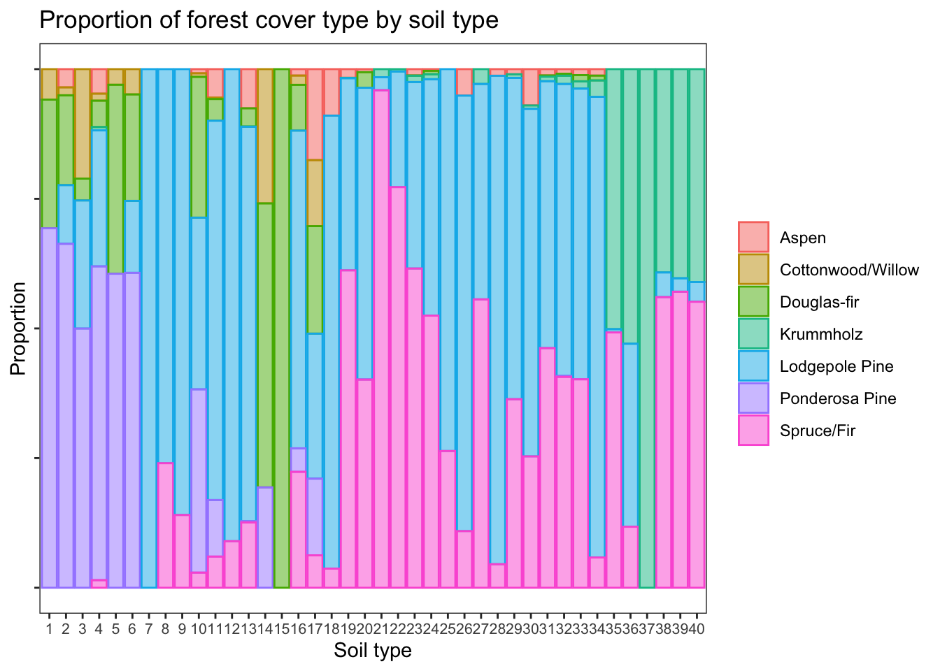
Proportion of forest cover types by soil type
d %>% ggplot(aes(soil_type, fill = cover, color = cover)) +
  geom_bar(alpha = 0.5, position = 'fill') +
  theme_bw() +
  labs(
    title = 'Proportion of forest cover type by soil type',
    x = 'Soil type', y = 'Proportion'
    ) +
  theme(
    panel.grid = element_blank(),
    axis.text.x = element_text(size = 8),
    legend.title = element_blank(),
    axis.text.y = element_blank()
    )
Forest cover by climatic zone
d %>% ggplot(aes(climate, fill = cover, color = cover)) +
  geom_bar(position = 'fill', alpha = 0.5) +
  labs(title = 'Proportion of Forest Cover by Climatic Zone', y = 'Proportion') +
  theme_bw() +
  theme(panel.grid = element_blank(), axis.text.x = element_text(angle=20, hjust = 1),
    legend.title = element_blank(), axis.title.x = element_blank())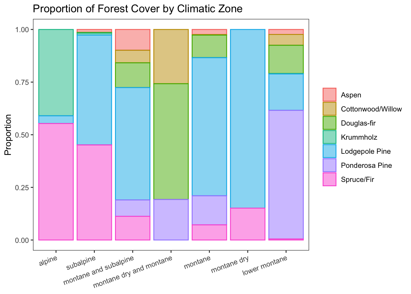
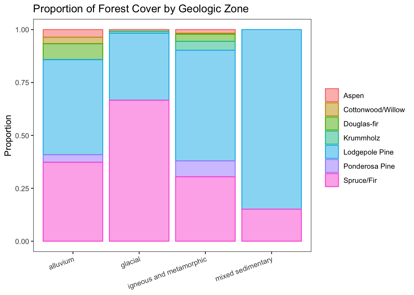
Forest cover by geologic zone
d %>% ggplot(aes(geologic, fill = cover, color = cover)) +
  geom_bar(position = 'fill', alpha = 0.5) +
  labs(title = 'Proportion of Forest Cover by Geologic Zone', y = 'Proportion') +
  theme_bw() +
  theme(
    panel.grid = element_blank(),
    axis.text.x = element_text(angle=20, hjust = 1),
    axis.title.x = element_blank(),
    legend.title = element_blank()
  )
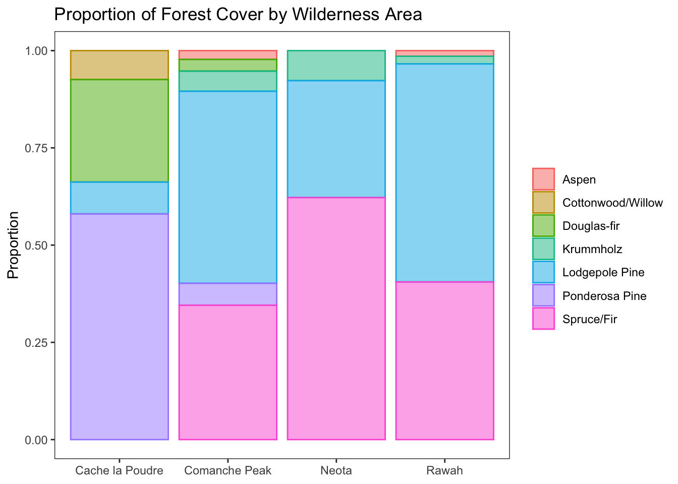
Forest cover by wilderness area
d %>% ggplot(aes(wilderness_type, fill = cover, color = cover)) +
  geom_bar(position = 'fill', alpha = 0.5) +
  labs(title = 'Proportion of Forest Cover by Wilderness Area', y = 'Proportion') +
  theme_bw() +
  theme(
    panel.grid = element_blank(),
    axis.title.x = element_blank(),
    legend.title = element_blank()
  )
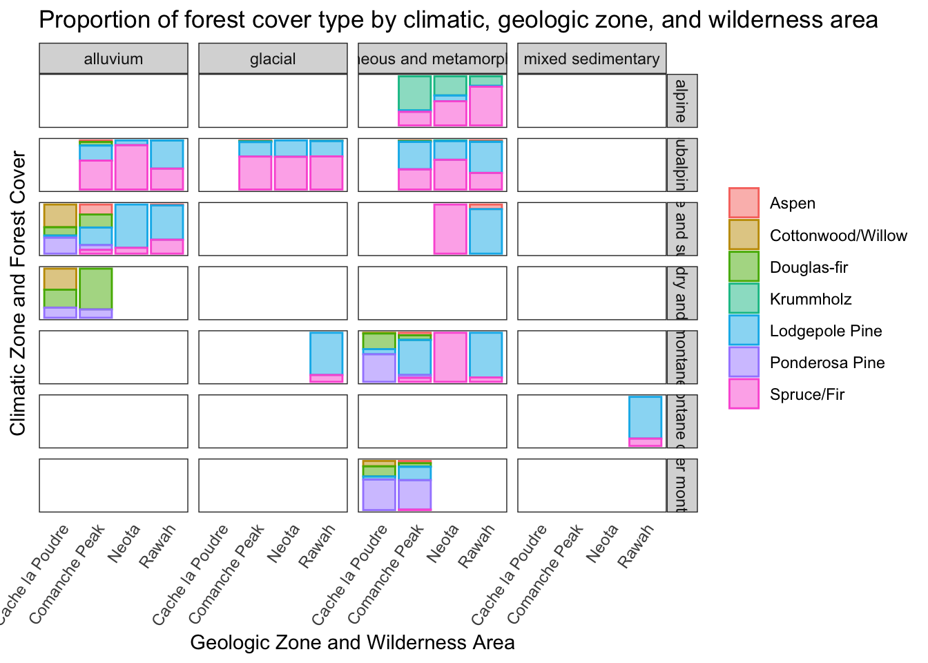
Proportion of forest cover type by climatic zone, geologic zone, and wilderness area
The following plot demonstrates the interactions between the target category and three different categorical predictors.
d %>% ggplot(aes(wilderness_type, fill = cover, color = cover)) +
  geom_bar(position = 'fill', alpha = 0.5) +
  facet_grid(climate ~ geologic) +
  theme_bw() +
  labs(
    title = 'Proportion of forest cover type by climatic, geologic zone, and wilderness area',
    y = 'Climatic Zone and Forest Cover', x = 'Geologic Zone and Wilderness Area'
    ) +
  theme(
    panel.grid = element_blank(),
    axis.text.x = element_text(angle=55, hjust = 1),
    legend.title = element_blank(),
    # axis.title.x = element_blank(),
    axis.text.y = element_blank(),
    # axis.text.x = element_blank(),
    axis.ticks = element_blank()
    )
Initial exploration of predictive modeling
Just for fun: Random Forests for Forest Cover Prediction
(It just seems right to use this particular model to predict this particular target, right?)
The data dictionary reports classification performance from ~1998, using the first 15,120 records used for training and validation, and the remaining 565,892 records for model performance testing, with the following classification accuracy:
- 70% Neural Network (backpropagation)
- 58% Linear Discriminant Analysis
Without doing proper cross-validation for determination of optimal hyperparameters, the first 15,120 records were used for training a Random Forest classifier.
A training set out-of-bag accuracy of 83.5% was obtained.
train <- d[c(1:15120), ]
test <- d[-c(1:15120), ]
rfmodel <- randomForest(cover ~ ., data = train, importance = TRUE, ntree = 300)
# save(rfmodel, file = 'rfmodel.Rda')
# load('rfmodel.Rda')
rfmodel
Call:
 randomForest(formula = cover ~ ., data = train, importance = TRUE,      ntree = 300)
               Type of random forest: classification
                     Number of trees: 300
No. of variables tried at each split: 3

        OOB estimate of  error rate: 12.95%
Confusion matrix:
                  Aspen Cottonwood/Willow Douglas-fir Krummholz Lodgepole Pine
Aspen              2062                 0          20         0             44
Cottonwood/Willow     0              2097          22         0              0
Douglas-fir           8                49        1907         0             17
Krummholz             0                 0           0      2091              5
Lodgepole Pine      149                 0          49        17           1538
Ponderosa Pine       19                88         234         0             10
Spruce/Fir           37                 0           3       123            337
                  Ponderosa Pine Spruce/Fir class.error
Aspen                         30          4  0.04537037
Cottonwood/Willow             41          0  0.02916667
Douglas-fir                  178          1  0.11712963
Krummholz                      0         64  0.03194444
Lodgepole Pine                49        358  0.28796296
Ponderosa Pine              1809          0  0.16250000
Spruce/Fir                     2       1658  0.23240741
Variable importance in random forest model
importance(rfmodel) %>%
  as.data.frame %>%
  cbind(list(names = row.names(importance(rfmodel)))) %>%
  select(c(10,8,9)) %>%
  arrange(desc(MeanDecreaseAccuracy))
names MeanDecreaseAccuracy MeanDecreaseGini
elevation elevation 82.05646 2932.6349
hydro_h hydro_h 76.21345 769.4528
shade_12 shade_12 68.13971 520.2648
road_h road_h 59.76714 1141.5291
fire_h fire_h 57.97839 953.2702
shade_09 shade_09 56.82135 643.0753
soil_type soil_type 55.83001 1486.8193
hydro_v hydro_v 53.17607 625.0303
shade_15 shade_15 52.53195 544.1503
aspect aspect 50.83801 597.2513
slope slope 39.22942 401.2883
wilderness_type wilderness_type 38.58556 759.7641
climate climate 35.37959 1368.8726
geologic geologic 24.12719 158.3731Accuracy on test set
Using the random forest model trained on the first 15,120 samples yielded a test set (remaining 565,892 samples) accuracy of 75.0%, similar to the performance of the neural network from ~1998. Optimizing model training would likely yield substantial improvements.
The difference in classification accuracy from the OOB training set and the test set seems a bit extreme. One possibility is that the ordering of the samples is NOT random, so choosing the first 15,120 samples may not be a representative sample.
pred <- predict(rfmodel, test)
sum(pred == test$cover) / nrow(test)
[1] 0.7539318