Vignette for the medianeffect R package for dose-effect analysis and quantifying synergism and antagonism via the Median Effect Principle.

Vignette for the medianeffect R package
The medianeffect R package implements methods for drug dose and effect analysis and quantifying degree of synergism versus antagonism via the Median Effect Principle (Chou, 1976; Chou and Talalay, 1984).
This work is neither approved nor endorsed by Dr. Ting-Chao Chou, the developer of this analytic approach.
In this document, the medianeffect package is used to replicate analysis from (Chou et al., 1994) reporting the effect of paclitaxel, cisplatin, and topotecan individually and in 2- and 3-drug combinations on inhibition of 833K teratocarcinoma cells. The drug dose-effect data is taken from Table 3.
After package installation, this document is available via vignette('medianeffect').
Setup
If not previously done, install the medianeffect package from GitHub):
devtools::install_github("jhchou/medianeffect", build_vignettes = TRUE)The package is made available under the permissive MIT open source license, allowing rights to use, copy, modify, merge, publish, distribute, sublicense, and/or sell copies of the Software, subject to attribution and inclusion of the MIT license notice in derivative works. The MIT license also limits any liability in connection with this Software.
Once installed, load the medianeffect package:
library(medianeffect)Single drug effects
Drug effect objects are then created with the drug_effects function. As each one is created, the dose-effect parameters (e.g., m and Dm) are calculated and stored with the object.
Displaying the object (with print(object) or just object interactively) shows the doses, effects, calculated m and Dm parameters, and the coefficient of determination (R^2) from the linear regression fit. Historically, R was also reported in median effect analysis, so it is included as well.
Single drug: paclitaxel
drug1 <- drug_effects(
  D = c(0.002, 0.004, 0.005, 0.01, 0.02),
  fa = c(0.429, 0.708, 0.761, 0.882, 0.932),
  name = "Paclitaxel",
  label = "Paclitaxel")
drug1
#> Paclitaxel (Paclitaxel)
#>
#> |     D|    fa|
#> |-----:|-----:|
#> | 0.002| 0.429|
#> | 0.004| 0.708|
#> | 0.005| 0.761|
#> | 0.010| 0.882|
#> | 0.020| 0.932|
#>
#> m: 1.247829
#> Dm: 0.002167772
#> R2: 0.9803665
#> R: 0.9901346
Single drug: cisplatin
drug2 <- drug_effects(
  D = c(0.05, 0.1, 0.2, 0.5, 1, 2),
  fa = c(0.055, 0.233, 0.301, 0.559, 0.821, 0.953),
  name = "Cisplatin",
  label = "cis-pt")
drug2
#> Cisplatin (cis-pt)
#>
#> |    D|    fa|
#> |----:|-----:|
#> | 0.05| 0.055|
#> | 0.10| 0.233|
#> | 0.20| 0.301|
#> | 0.50| 0.559|
#> | 1.00| 0.821|
#> | 2.00| 0.953|
#>
#> m: 1.4599
#> Dm: 0.3201557
#> R2: 0.9721869
#> R: 0.9859954
Single drug: topotecan
drug3 <- drug_effects(
  D = c(0.01, 0.02, 0.05, 0.1, 0.2, 0.5),
  fa = c(0.069, 0.213, 0.373, 0.785, 0.94, 0.991),
  name = 'Topotecan',
  label = 'Topotecan'
)
drug3
#> Topotecan (Topotecan)
#>
#> |    D|    fa|
#> |----:|-----:|
#> | 0.01| 0.069|
#> | 0.02| 0.213|
#> | 0.05| 0.373|
#> | 0.10| 0.785|
#> | 0.20| 0.940|
#> | 0.50| 0.991|
#>
#> m: 1.854857
#> Dm: 0.04621344
#> R2: 0.9821425
#> R: 0.991031
Multi-drug combination effects
Next, the 2- and 3-drug constant ratio combination drug effect objects are created, also using the drug_effects function, but now specifying the ratio of doses between the different drugs. The doses entered are the sum of all the doses, and the ratio is used to calculate the individual drug dose contributions.
If the sum of the doses is not known, R vector addition can be used to generate the sums, as done here.
Two-drug constant ratio combination: paclitaxel and cisplatin
combo_1_2 <- drug_effects(
  D = c(0.001, 0.002, 0.005, 0.01) + c(0.1, 0.2, 0.5, 1),
  fa = c(0.45, 0.701, 0.910, 0.968),
  name = 'Paclitaxel - Cisplatin',
  label = 'taxol:cispt',
  ratio = c(0.001, 0.1))
combo_1_2
#> Paclitaxel - Cisplatin (taxol:cispt)
#> Drug ratio: 1 : 100
#>
#> |     D|    fa| drug_1| drug_2|
#> |-----:|-----:|------:|------:|
#> | 0.101| 0.450|  0.001|    0.1|
#> | 0.202| 0.701|  0.002|    0.2|
#> | 0.505| 0.910|  0.005|    0.5|
#> | 1.010| 0.968|  0.010|    1.0|
#>
#> m: 1.571597
#> Dm: 0.1159 = 0.001147 + 0.1147
#> R2: 0.9999033
#> R: 0.9999517
Two-drug constant ratio combination: cisplatin and topotecan
combo_2_3 <- drug_effects(
  D = c(0.05, 0.1, 0.2, 0.5, 1) + c(0.005, 0.01, 0.02, 0.05, 0.1),
  fa = c(0.304, 0.413, 0.675, 0.924, 0.977),
  name = 'Cisplatin - Topotecan',
  label = 'combo_2_3',
  ratio = c(0.1, 0.01))
combo_2_3
#> Cisplatin - Topotecan (combo_2_3)
#> Drug ratio: 10 : 1
#>
#> |     D|    fa| drug_1| drug_2|
#> |-----:|-----:|------:|------:|
#> | 0.055| 0.304|   0.05|  0.005|
#> | 0.110| 0.413|   0.10|  0.010|
#> | 0.220| 0.675|   0.20|  0.020|
#> | 0.550| 0.924|   0.50|  0.050|
#> | 1.100| 0.977|   1.00|  0.100|
#>
#> m: 1.587817
#> Dm: 0.1159 = 0.1053 + 0.01053
#> R2: 0.9790727
#> R: 0.989481
Two-drug constant ratio combination: paclitaxel and topotecan
combo_1_3 <- drug_effects(
  D = c(0.001, 0.002, 0.005, 0.01) + c(0.01, 0.02, 0.05, 0.1),
  fa = c(0.274, 0.579, 0.901, 0.965),
  name = 'Paclitaxel - Topotecan',
  label = 'combo_1_3',
  ratio = c(0.01, 0.1))
combo_1_3
#> Paclitaxel - Topotecan (combo_1_3)
#> Drug ratio: 1 : 10
#>
#> |     D|    fa| drug_1| drug_2|
#> |-----:|-----:|------:|------:|
#> | 0.011| 0.274|  0.001|   0.01|
#> | 0.022| 0.579|  0.002|   0.02|
#> | 0.055| 0.901|  0.005|   0.05|
#> | 0.110| 0.965|  0.010|   0.10|
#>
#> m: 1.89081
#> Dm: 0.01827 = 0.001661 + 0.01661
#> R2: 0.9979241
#> R: 0.9989615
Three-drug constant ratio combination: paclitaxel, cisplatin, and topotecan
A three-drug combination object is generated by changing the ratio term to include 3 elements.
combo_1_2_3 <- drug_effects(
  D = c(0.001, 0.002, 0.003, 0.005) + c(0.1, 0.2, 0.3, 0.5) + c(0.01, 0.02, 0.03, 0.05),
  fa = c(0.456, 0.806, 0.947, 0.995),
  name = 'Paclitaxel - Cisplatin - Topotecan',
  label = 'combo_1_2_3',
  ratio = c(0.001, 0.1, 0.01))
combo_1_2_3
#> Paclitaxel - Cisplatin - Topotecan (combo_1_2_3)
#> Drug ratio: 1 : 100 : 10
#>
#> |     D|    fa| drug_1| drug_2| drug_3|
#> |-----:|-----:|------:|------:|------:|
#> | 0.111| 0.456|  0.001|    0.1|   0.01|
#> | 0.222| 0.806|  0.002|    0.2|   0.02|
#> | 0.333| 0.947|  0.003|    0.3|   0.03|
#> | 0.555| 0.995|  0.005|    0.5|   0.05|
#>
#> m: 3.363359
#> Dm: 0.1289 = 0.001162 + 0.1162 + 0.01162
#> R2: 0.9683554
#> R: 0.9840505
Plots
Dose effect and median effect (linearized) plots can be generated for any number of the drug_effect objects created above. (However, attempting to plot more than 6 objects simultaneously is not recommended, as there are not enough point shapes available.)
Median effect plots
To generate a median effect plot (\(log\left(\frac{f_a}{1 - f_a}\right)\) versus \(log(D)\)), from which the Dm and m parameters were calculated after fitting a linear regression, use the median_effect_plot function and pass in any number of drug_effects objects.
For example, for a plot of just paclitaxel:
median_effect_plot(drug1)
#> `geom_smooth()` using formula 'y ~ x'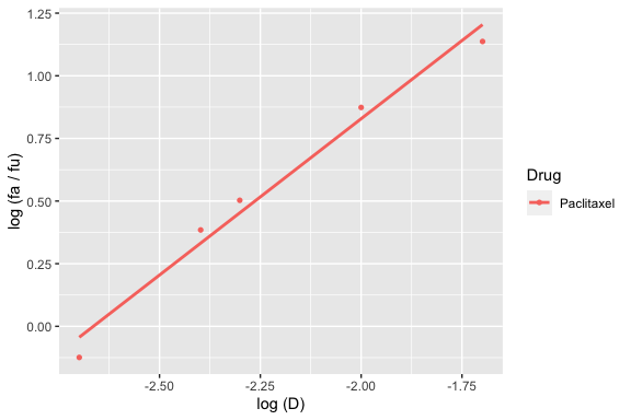
And to plot paclitaxel, cisplatin, and the paclitaxel:cisplatin combination:
median_effect_plot(drug1, drug2, combo_1_2)
#> `geom_smooth()` using formula 'y ~ x'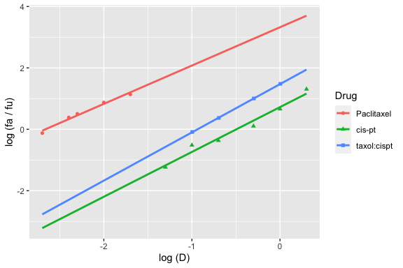
Dose-effect plots
Similarly, dose-effect plots (\(f_a\) versus \(D\), not linearized) can be generated with the dose_effect_plot function:
dose_effect_plot(drug1, drug2, combo_1_2)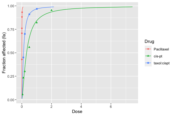
For more advanced R users, modifications can be performed on the plot. For example, the above plot extends to doses that may be too high. Two possible ways to handle this are shown below.
First, you can restrict the fa values to be used by the dose_effect_plot function (defaults to from 0.01 to 0.99), by modifying the from, to, and by parameters. However, this results in an unpleasant truncation of the higher effects.
dose_effect_plot(drug1, drug2, combo_1_2, from = 0.01, to = 0.95)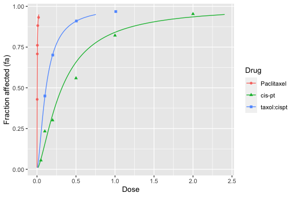
A better way is to know that dose_effect_plot and median_effect_plot return R ggplot objects, which can then be modified. The following limits the X axis to between 0 and 3:
dose_effect_plot(drug1, drug2, combo_1_2) + ggplot2::coord_cartesian(xlim = c(0, 3))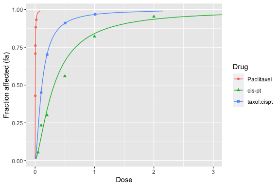
Drug combination analysis
fa-CI plot
fa-CI plots can be generated with the fa_ci_plot function, by passing in a drug combination object followed by the single drug objects. The order of the single drug objects must match the order defined by the ratio parameter.
The following is the fa-CI plot for the 3-drug combination:
fa_ci_plot(combo_1_2_3, drug1, drug2, drug3)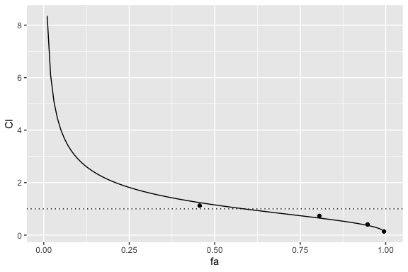
Knowledge of ggplot objects can allow axis transformations. For example, the following displays the Y-axis on a base 10 log scale:
fa_ci_plot(combo_1_2_3, drug1, drug2, drug3) + ggplot2::scale_y_continuous(trans='log10')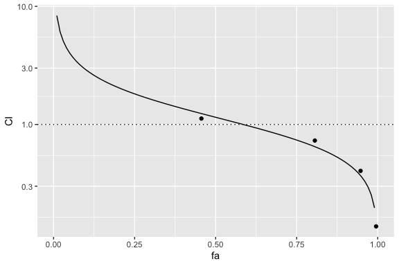
fa-DRI plot
Dose reduction index (DRI) plots are generated analogously, with the fa_dri_plot function. Below is an fa-DRI plot with the Y-axis on a log scale.
fa_dri_plot(combo_1_2_3, drug1, drug2, drug3) + ggplot2::scale_y_continuous(trans='log10')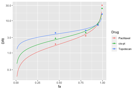
Calculations of CI and DRI at specified fa
The actual CI and DRI values can be displayed with the calc_ci and calc_dri functions. If no fa are specified, the calculations are performed at the fa observed in the combination.
3-drug combination CI at observed fa
calc_ci(combo_1_2_3, drug1, drug2, drug3)
#> # A tibble: 4 × 2
#>      fa    CI
#>   <dbl> <dbl>
#> 1 0.456 1.12
#> 2 0.806 0.731
#> 3 0.947 0.405
#> 4 0.995 0.137
3-drug combination DRI at observed fa
calc_dri(combo_1_2_3, drug1, drug2, drug3)
#> # A tibble: 4 × 4
#>      fa dri_drug_1 dri_drug_2 dri_drug_3
#>   <dbl>      <dbl>      <dbl>      <dbl>
#> 1 0.456       1.88       2.84       4.20
#> 2 0.806       3.39       4.25       4.98
#> 3 0.947       7.28       7.69       7.29
#> 4 0.995      30.2       24.0       16.0
Or, specific fa values can be provided to generate the numbers seen in Table 4.
CI for 3-drug combination at fa = 50% / 75% / 90% / 95%
calc_ci(combo_1_2_3, drug1, drug2, drug3, fa = c(0.5, 0.75, 0.9, 0.95))
#> # A tibble: 4 × 2
#>      fa    CI
#>   <dbl> <dbl>
#> 1  0.5  1.15
#> 2  0.75 0.738
#> 3  0.9  0.480
#> 4  0.95 0.361
DRI for 3-drug combination at fa = 50% / 75% / 90% / 95%
calc_dri(combo_1_2_3, drug1, drug2, drug3, fa = c(0.5, 0.75, 0.9, 0.95))
#> # A tibble: 4 × 4
#>      fa dri_drug_1 dri_drug_2 dri_drug_3
#>   <dbl>      <dbl>      <dbl>      <dbl>
#> 1  0.5        1.87       2.76       3.98
#> 2  0.75       3.25       4.22       5.19
#> 3  0.9        5.65       6.46       6.77
#> 4  0.95       8.23       8.63       8.11
Non-constant ratio combination analysis
Although not done in the cited study, the medianeffect package also supports calculations for drug combinations that are not at a constant ratio between drug components.
Combination index at observed fa
A non-constant ratio drug effect object is created with the ncr_drug_effects function, which takes vectors of each drug in the combination, followed by a vector of observed fraction affected.
# Create a 'fake' non-constant ratio object for testing
ncr_combo <- ncr_drug_effects(
  c(0.001, 0.002, 0.005, 0.01),
  c(0.1, 0.2, 0.5, 1),
  fa = c(0.45, 0.701, 0.910, 0.968),
  name='NCR Paclitaxel - Cisplatin',
  label = 'ncr_combo_1_2'
)
ncr_combo
#> NCR Paclitaxel - Cisplatin (ncr_combo_1_2)
#>
#> |    fa| drug_1| drug_2|
#> |-----:|------:|------:|
#> | 0.450|  0.001|    0.1|
#> | 0.701|  0.002|    0.2|
#> | 0.910|  0.005|    0.5|
#> | 0.968|  0.010|    1.0|
The combination index can then be calculated, but only for the observed fractional effects, using the ncr_calc_ci function:
ncr_calc_ci(ncr_combo, drug1, drug2)
#> # A tibble: 4 × 2
#>      fa    CI
#>   <dbl> <dbl>
#> 1 0.45  0.900
#> 2 0.701 0.815
#> 3 0.91  0.681
#> 4 0.968 0.602
Isobologram
Both standard and normalized isobologram plots can be generated using the isobologram_plot function, from two drug combinations at either constant or non-constant ratio, by passing in a two-drug drug combination object followed by two single drug objects.
Normalized isobologram (default)
isobologram_plot(combo_1_2, drug1, drug2)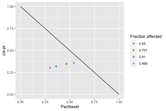
Standard isobologram
isobologram_plot(combo_1_2, drug1, drug2, normalized = FALSE)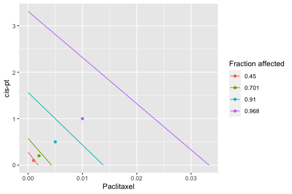
Appendix: Theoretical background
Median effect equation
The median effect equation (Chou, 1976) relates dose (D) to fraction affected (fa).
\[\frac{f_a}{f_u} = \left(\frac{D}{D_m}\right)^m\]
… where fraction affected plus fraction unaffected equals one, so: \(f_u = 1 - f_a\)
Dm parameter
At a dose of \(D = D_m\), the fraction affected will equal 50%; hence “median effect.”
m parameter
The \(m\) parameter describes the shape of the dose-effect relationship:
- \(m = 1\): hyperbolic
- \(m > 1\): sigmoidal
- \(m < 1\): negative (flat) sigmoidal
Linearizing by log transformation
\[log\left(\frac{f_a}{1 - f_a}\right) = m~log(D) - m~log(D_m)\]
Fitting a linear regression of \(log\left(\frac{f_a}{1 - f_a}\right)\) versus \(log(D)\) allows determination of the \(m\) and \(D_m\) parameters.
Solving for dose, D
\[D = D_m\left[\frac{f_a}{1 - f_a}\right]^{1/m}\]
Solving for fraction affected, fa
\[f_a = \frac{1}{1 + \left(\frac{D_m}{D}\right)^m}\]
Combination Index (CI)
The combination index (Chou and Talalay, 1984) describes the degree of synergism / antagonism, at a given fraction affected:
- CI = 1 indicates additive effect
- CI < 1 indicates synergism
- CI > 1 indicates antangonism
\[CI = \sum_{i=1}^{n} \frac{(D)_i}{(D_x)_i}\]
… where for a given fraction affected \(f_a\),
- \((D)_i\) is the dose of drug i within the combination of n drugs which together results in the fraction affected
- \((D_x)_i\) is the dose of drug i alone which results in the fraction affected = \(f_a\)
Dose reduction index (DRI)
\[DRI_i = \frac{(D_x)_i}{(D)_i}\]
The reciprocal of each of the terms of the combination index (CI) reflects the fold-reduction (dose reduction index, DRI) of drug i within the drug combination, at a given fractional affect \(f_a\).
Isobologram
The isobologram is a visualization method to assess combinations of two drugs. It has been asserted to be appropriate when the the effects of the drugs are mutually exclusive (Chou and Talalay, 1984).
Each axis reflects the dose of one of the two drugs and the plotted line indicates a predicted equipotency curve for additive effect. Plotted points for observed effects from a drug combination that fall above or below the equipotency curve reflect antagonism and synergism respectively.
In the standard isobologram, the X and Y axis reflect actual drug doses so a different line is plotted for each equipotency curve. The normalized isobologram standardizes the single drug doses to a value of 1 for all fractional effects, so all predicted additive equipotency curves are represented by a single line.
The medianeffect R package is limited to plotting isobolograms for two drug combinations, as more drugs would require plotting in higher dimensional space.