library(tidyverse) # https://www.tidyverse.org; https://r4ds.had.co.nz
library(tidytext)  # Julia Silge and David Robinson; https://www.tidytextmining.com
library(glmnet)    # Jerome Friedman et al; https://cran.r-project.org/web/packages/glmnet/glmnet.pdf

seed <- 1           # random seed called before glmnet cross-validation
num_features <- 300 # set approximate number of (word) features to select, via lambda for regularizationI attended a Greater Boston useR Group (R Programming Language) Meetup yesterday, where the topic was to work on a Tidy Tuesday dataset. This week was a wine-enthusiast ratings dataset from Kaggle.
I adapted some code I had previously written for a clinical dataset to analyze the text of the wine descriptions to predict wine scores. There was some interest in seeing the code I used, so I’m posting it here. I tried to include some explanatory comments in the code.
Would you rather have wine described with words like: “stunning, gorgeous, long, complex, beautiful, beautifully, superb, impressive, vineyard, years, beauty, decade, delicious, velvety, powerful”?
Or instead, with: “aromas, easy, tastes, sour, strange, lean, rustic, short, flat, bitter, thin, lacks, soft, simple, flavors”?
These were some of the positive and negative features identified.
Overall approach:
- use
tidytextto tokenize all the words and generate term frequency-inverse document frequency (TF-IDF) scores for each word in each wine description - the predictor matrix ends up pretty large, with 129,971 rows (wines) and ~31,000 prediction features (unique words)
- use
glmnetto generate a linear regression model to predict wine scores, using LASSO (L1) regularization to perform feature selection on the word features, and cross-validation to identify an appropriate regularization strength to result in a reasonable number of word features
This would also be an easy way to identify useful word features for sentiment analysis of wine reviews.
Predict point score by regularized linear regression using TF-IDF of descriptions
Setup and data loading
# Tidy Tuesday: https://github.com/rfordatascience/tidytuesday
# - 2019-05-28 dataset: https://github.com/rfordatascience/tidytuesday/tree/master/data/2019/2019-05-28
# - dataset from: https://www.kaggle.com/zynicide/wine-reviews
wine <- read.csv("winemag-data-130k-v2.csv", stringsAsFactors = FALSE)
names(wine)[1] <- 'id' # give the unique identifier column a name
Prep dataset
Simplify dataset to dataframe with only 3 columns:
id: unique idtext: source of textoutcome_target: outcome target to predict
df <- wine %>%
  transmute(
    id = as.character(id),  # will use for table joins
    text = description,     # source of text
    outcome_target = points # define the outcome target: points + price for continuous, but price is very skewed
  ) %>%
  filter(!is.na(outcome_target)) # glmnet will fail if any missing values

# df <- df %>% sample_n(1500) # if don't want to train on full 129,000+ wine dataset...
Distribution of outcome target
df %>% ggplot(aes(outcome_target)) + geom_histogram(color = 'black', fill = 'grey', binwidth = 1) + theme_bw()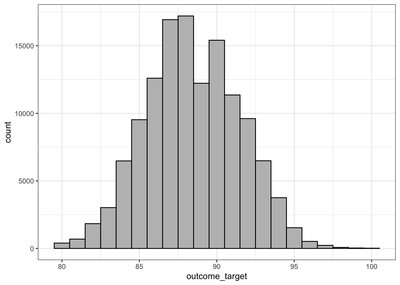
Tidy text
- Tokenize the text to lowercase words, remove numbers, remove stopwords
- Output is for each unique id, the count of each word feature
tidy <- df %>%
  select(id, text) %>%
  unnest_tokens(word, text) %>% # tidytext tokenize text to lowercase words
  mutate(word = str_extract(word, "[a-z']+")) %>% # greedy matches first string of [a-z] of length at least 1, removing trailing non-letters
  filter(!is.na(word)) %>% # all those tokens which had NO [a-z] characters, like numbers
  anti_join(get_stopwords(), by = 'word') %>% # remove stopwords
count(id, word, sort = TRUE)head(tidy) ## Count of each unique word token for each id id word n
1 54963 black 6
2 106687 white 5
3 11616 white 5
4 127916 cherry 5
5 20435 wine 5
6 34198 white 5What are the most common words in the entire corpus?
tidy %>% group_by(word) %>% summarise(n = sum(n)) %>% arrange(desc(n)) %>% head()# A tibble: 6 × 2
word n
<chr> <int>
1 wine 78337
2 flavors 62795
3 fruit 49928
4 aromas 39639
5 palate 38437
6 acidity 35003Calculate tf, idf, and tf-idf values
tidy_tf_idf <- tidy %>%
  bind_tf_idf(word, id, n) # for each id / word, calculate n, tf, idf, tf_idf

head(tidy_tf_idf)
id word n tf idf tf_idf
1 54963 black 6 0.1538462 1.6700270 0.2569272
2 106687 white 5 0.1282051 2.4124344 0.3092865
3 11616 white 5 0.2173913 2.4124344 0.5244423
4 127916 cherry 5 0.2173913 1.5563670 0.3383406
5 20435 wine 5 0.1388889 0.7209121 0.1001267
6 34198 white 5 0.2173913 2.4124344 0.5244423Add rows which contain the outcome target
# - a little kludgy -- will force the outcomes into the same 3 columns as tidy_tf_idf's, so can bind_rows
# - for each 'id', the 'word' will be 'outcome_target' and the 'tf_idf' will be the prediction target
# - will later pull this out as the vector 'y' prediction target
tidy_tf_idf <- tidy_tf_idf %>%
  bind_rows(
    df %>% transmute(
      id = id,
      word = 'outcome_target',
      tf_idf = outcome_target
    )
  )
Convert from tidy long format to sparse matrix and prediction target vector for glmnet
- each row is a unique wine: n = 129,971
- each column is a word feature: n = tens of thousands
- this is a huge matrix – since word features are sparse, will cast to a sparse matrix
# Cast to sparse matrix
sp <- cast_sparse(tidy_tf_idf, row = id, column = word, value = tf_idf)
sp <- sp[, c(which(colnames(sp)=="outcome_target"), which(colnames(sp) != "outcome_target"))] # move 'outcome_target' to first column
dimnames(sp)[[2]] %>% head # confirm column names, with 'outcome_target' moved to first column; each column is a unique predictor word token
[1] "outcome_target" "black" "white" "cherry"
[5] "wine" "orange" x <- sp[, 2:dim(sp)[2]] # predictor matrix, all but the first column
y <- as.numeric(sp[, 1]) # outcome vector of point scores, from the first column
dim(x) # sparse matrix of dimensions: # of documents x # of unique word tokens[1] 129971 31725glmnet elasticnet model building, using cross-validation to choose regularization strength
- primarily LASSO regularization, to get feature selection and not just coefficient shrinkage
##### Fit glmnet elasticnet model #####
set.seed(seed)
# degree of L1 versus L2 regularization -- glmnet: alpha = 0.99 'performed much like the lasso, but removes any degeneracies ... caused by extreme correlations'
cvfit = cv.glmnet(x, y, type.measure = "mse", alpha = 0.99, nfolds = 10) # primarily LASSO, to get feature selection
# cvfit = cv.glmnet(x, y, family = "binomial", type.measure = "auc", alpha = 0.99, nfolds = 20) # if wanted binary classification, logistic regression, maximizing AUC
Result of search for optimal lambda for regularization
- on top of plot, show numbers of non-zero coeffecients (i.e., number of word predictors selected)
# Not going to use lambdas that minimize the cost function, because with the wine dataset, selects too many features
# cvfit$lambda.min # lambda resulting minimizing cost function
# cvfit$lambda.1se # typically use 1 standard error from minimum
plot(cvfit) # cross-validation search for optimal lambda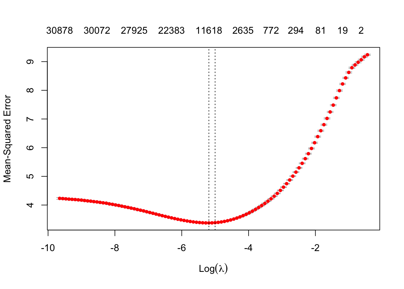
# create a dataframe of tested lambdas, number of predictors, and list of predictors at each lambda
len = length(cvfit$lambda)
predictors_select <- tibble(lambda = cvfit$lambda, nzero = cvfit$nzero, features = vector('character', len))
for (i in 1:len) {
  index_list <- which(coef(cvfit, s = predictors_select$lambda[i]) != 0) # indices of the predictor columns to keep
  temp <- tibble( # features by decreasing magnitude; outcome_target is the intercept term
    word = colnames(sp)[index_list],
    beta = coef(cvfit, s = cvfit$lambda[i])[index_list]
  ) %>%
  arrange(desc(abs(beta)))
  predictors_select$features[i] <- paste(temp$word, collapse = '#')
}
Choose a lambda regularization strength that generates a desired approximate number of selected features
lambda_num_features <- predictors_select %>% # find the maximum lambda that generates at least num_features features
  arrange(desc(lambda)) %>%
  filter(nzero >= num_features) %>%
  .$lambda %>%
  max()

lambda_num_features
[1] 0.0688468Plot of number of predictors selected versus increasing regularization lambda
predictors_select %>%
  filter(nzero != 0) %>%
  ggplot(aes(lambda, nzero)) +
  geom_point() +
  geom_vline(xintercept = cvfit$lambda.min, color = 'red') +
  geom_vline(xintercept = cvfit$lambda.1se, color = 'orange') +
  geom_vline(xintercept = lambda_num_features, color = 'blue') +
  scale_x_continuous(trans='log10') +
  scale_y_continuous(trans='log10') +
  labs(y = 'Number of features selected') +
  theme_bw()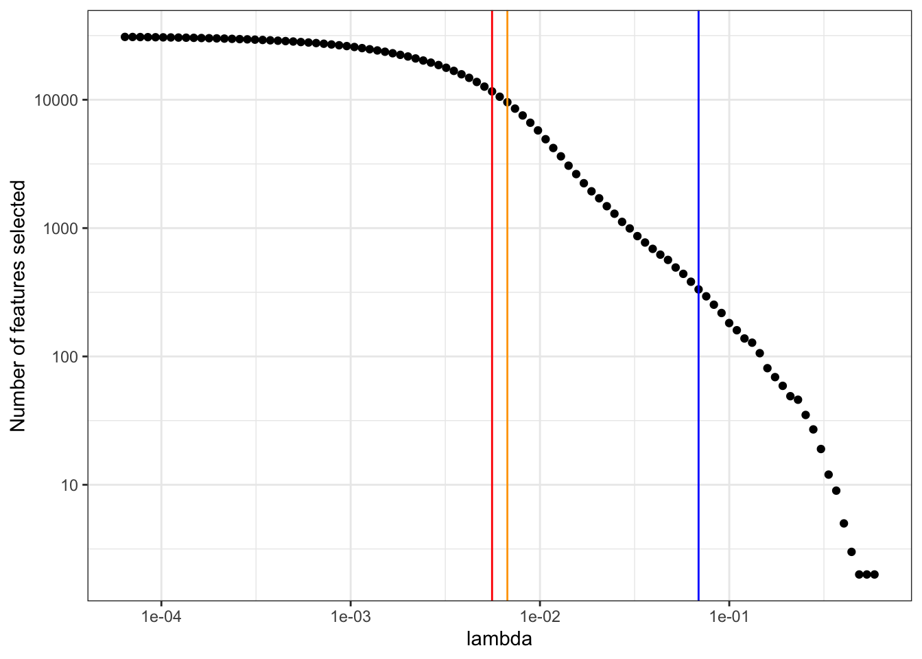
Generate a dataframe that fully describes the model
- contains the word features selected, the beta coefficients, and the inverse document frequency of that term within the training corpus
- (if wanted to do predictions on new data, would need to normalize the term frequencies to the IDF of the training corpus)
optimal_lambda <- lambda_num_features

# create data frame of predictors, coefficients, and idf values, sorted by decreasing coefficient
indices <- which(coef(cvfit, s = optimal_lambda) != 0) # indices of the predictor columns to keep
predictors <- tibble( # display predictors by decreasing magnitude; outcome_target is the intercept term
    word = colnames(sp)[indices],
    beta = coef(cvfit, s = optimal_lambda)[indices]
  ) %>%
  left_join( # Get the IDF's for the chosen terms, to be able to apply model to future datasets
    tidy_tf_idf %>% filter(word %in% colnames(sp)[indices]) %>% select(word, idf) %>% unique,
    by = 'word'
  ) %>%
  arrange(desc(beta))
Predictors with the most positive coefficients (associated with a high outcome_target)
head(predictors %>% filter(word != 'outcome_target'), n = 10)# A tibble: 10 × 3
word beta idf
<chr> <dbl> <dbl>
1 stunning 9.99 6.13
2 gorgeous 8.84 5.26
3 long 8.35 3.02
4 complex 8.25 3.32
5 beautiful 7.99 4.43
6 beautifully 7.21 4.51
7 superb 7.14 6.18
8 impressive 6.92 4.26
9 vineyard 6.75 3.10
10 years 6.33 2.85Predictors with the most negative coefficients (associated with a low outcome_target)
tail(predictors, n = 10)# A tibble: 10 × 3
word beta idf
<chr> <dbl> <dbl>
1 lean -4.67 4.02
2 rustic -4.69 4.57
3 short -4.76 4.60
4 flat -5.03 5.08
5 bitter -5.41 3.69
6 thin -5.47 4.94
7 lacks -5.78 5.04
8 soft -5.91 2.28
9 simple -7.92 3.53
10 flavors -13.8 0.779Make predictions
pred <- predict(cvfit, s = optimal_lambda, newx = x)Root mean square error of predictions
df <- df %>%
  left_join(
    tibble(id = rownames(pred), prediction = pred[,1]), # add column of predictions
    by = 'id'
  )

sqrt(mean((df$outcome_target - df$prediction)^2))
[1] 2.231615Plot of predictions versus actual target
- the black line would represent perfect prediction
- the lower slope of the model (blue line) suggests an underestimate of prediction at higher target values
- not sure why the slope isn’t one
df %>%
  sample_n(1000) %>%
  ggplot(aes(outcome_target, prediction)) +
  geom_jitter(size = 0.3) +
  geom_smooth(method = 'lm', se = FALSE) +
  geom_abline(slope = 1, intercept = 0) +
  theme_bw()
`geom_smooth()` using formula 'y ~ x'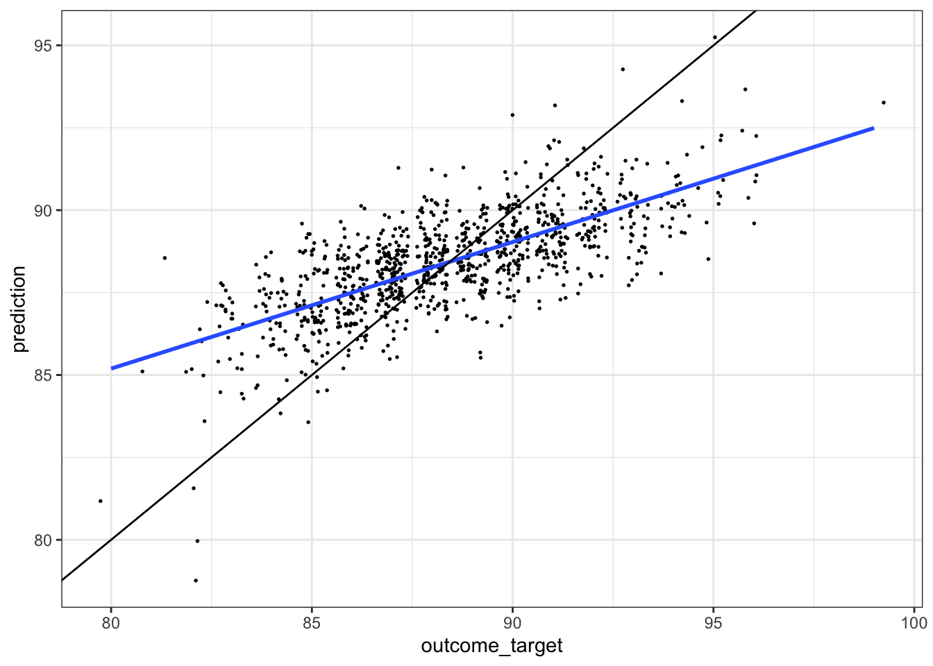
Other thoughts
- do different varieties of wine have different word features? E.g., perhaps ‘sweet’ might be good for a dessert wine, but not so good for a red wine?
- do different reviewers systematically use words differently?
- is there a good way to combine other features with the TF-IDF matrix of description text, to improve model performance?
- (even with this TF-IDF model, the cross validation suggests using ~10,000 word features would improve performance, without overfitting, but that seems unlikely)
- to predict on new data, need to use IDF scores of the training corpus, and need additional code to create a feature matrix that includes all word features of the model, even if not present in the new data